
3. From Neural Architecture Search to Automated Deep Ensemble with Uncertainty Quantification#
[ ]:
!pip install deephyper["autodeuq"]
3.1. Imports and GPU Detection#
[1]:
import json
import os
import pathlib
import shutil

!export TF_CPP_MIN_LOG_LEVEL=3
!export TF_XLA_FLAGS=--tf_xla_enable_xla_devices

import matplotlib.pyplot as plt
import numpy as np
import tensorflow as tf
Note
The TF_CPP_MIN_LOG_LEVEL can be used to avoid the logging of Tensorflow DEBUG, INFO and WARNING statements.
Note
The following can be used to detect if GPU devices are available on the current host.
[2]:
available_gpus = tf.config.list_physical_devices("GPU")
n_gpus = len(available_gpus)
if n_gpus > 1:
    n_gpus -= 1
is_gpu_available = n_gpus > 0

if is_gpu_available:
    print(f"{n_gpus} GPU{'s are' if n_gpus > 1 else ' is'} available.")
else:
    print("No GPU available")
No GPU available
3.2. Start Ray#
We launch the Ray run-time depending on the detected local ressources. If GPU(s) is(are) detected then 1 worker is started for each GPU. If not, then only 1 worker is started. You can start more workers by setting num_cpus=1 to a value greater than 1.
Warning
In the case of GPUs it is important to follow this scheme to avoid multiple processes (Ray workers vs current process) to lock the same GPU.
[3]:
import ray

if not(ray.is_initialized()):
    if is_gpu_available:
        ray.init(num_cpus=n_gpus, num_gpus=n_gpus, log_to_driver=False)
    else:
        ray.init(num_cpus=4, log_to_driver=False)
3.3. A Synthetic Dataset#
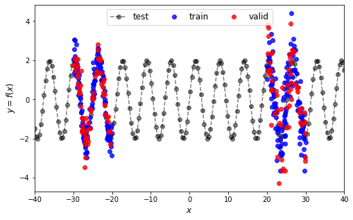
Now, we will start by defining our artificial dataset based on a Sinus curve. We will first generate data for a training set (used for estimation) and a testing set (used to evaluate the final performance). Then the training set will be sub-divided in a new training set (used to estimate the neural network weights) and validation set (used to estimate the neural network hyperparameters and architecture). The data are generated from the following function:
The training data will be generated in a range between \([-30, -20]\) with \(\epsilon \sim \mathcal{N}(0,0.25)\) and in a range between \([20, 30]\) with \(\epsilon \sim \mathcal{N}(0,1)\). The code for the training data is then corresponding to:
[4]:
def load_data_train_test(random_state=42):
    rs = np.random.RandomState(random_state)

    train_size = 400
    f = lambda x: 2*np.sin(x) # a simlpe affine function

    x_1 = rs.uniform(low=-30, high=-20.0, size=train_size//2)
    eps_1 = rs.normal(loc=0.0, scale=0.5, size=train_size//2)
    y_1 = f(x_1) + eps_1

    x_2 = rs.uniform(low=20.0, high=30.0, size=train_size//2)
    eps_2 = rs.normal(loc=0.0, scale=1.0, size=train_size//2)
    y_2 = f(x_2) + eps_2

    x = np.concatenate([x_1, x_2], axis=0)
    y = np.concatenate([y_1, y_2], axis=0)

    x_tst = np.linspace(-40.0, 40.0, 200)
    y_tst = f(x_tst)

    x = x.reshape(-1, 1)
    y = y.reshape(-1, 1)

    x_tst = x_tst.reshape(-1, 1)
    y_tst = y_tst.reshape(-1, 1)

    return (x, y), (x_tst, y_tst)
Then the code to split the training data in a new training set and a validation set corresponds to:
[5]:
from sklearn.model_selection import train_test_split

def load_data_train_valid(verbose=0, random_state=42):

    (x, y), _ = load_data_train_test(random_state=random_state)

    train_X, valid_X, train_y, valid_y = train_test_split(
        x, y, test_size=0.33, random_state=random_state
    )

    if verbose:
        print(f'train_X shape: {np.shape(train_X)}')
        print(f'train_y shape: {np.shape(train_y)}')
        print(f'valid_X shape: {np.shape(valid_X)}')
        print(f'valid_y shape: {np.shape(valid_y)}')
    return (train_X, train_y), (valid_X, valid_y)


(x, y), (vx, vy) = load_data_train_valid(verbose=1)
_, (tx , ty) = load_data_train_test()
train_X shape: (268, 1)
train_y shape: (268, 1)
valid_X shape: (132, 1)
valid_y shape: (132, 1)
Note
When it is possible to factorize the two previous function into one, DeepHyper interface requires a function which returns (train_inputs, train_outputs), (valid_inputs, valid_outputs).
We can give a visualization of this data:
[6]:
width = 8
height = width/1.618
plt.figure(figsize=(width, height))

plt.plot(tx.reshape(-1), ty.reshape(-1), "ko--", label="test", alpha=0.5)
plt.plot(x.reshape(-1), y.reshape(-1), "bo", label="train", alpha=0.8)
plt.plot(vx.reshape(-1), vy.reshape(-1), "ro", label="valid", alpha=0.8)

plt.ylabel("$y = f(x)$", fontsize=12)
plt.xlabel("$x$", fontsize=12)

plt.xlim(-40, 40)
plt.legend(loc="upper center", ncol=3, fontsize=12)

plt.show()
3.4. Scaling the Data#
It is important to apply standard scaling on the input/output data to have faster convergence when training.
[7]:
from sklearn.preprocessing import StandardScaler


scaler_x = StandardScaler()
s_x = scaler_x.fit_transform(x)
s_vx = scaler_x.transform(vx)
s_tx = scaler_x.transform(tx)

scaler_y = StandardScaler()
s_y = scaler_y.fit_transform(y)
s_vy = scaler_y.transform(vy)
s_ty = scaler_y.transform(ty)
3.5. Baseline Neural Network#
Let us define a baseline neural network based on a regular multi-layer perceptron architecture which learn the mean estimate and minimise the mean squared error.
[8]:
input_ = tf.keras.layers.Input(shape=(1,))
out = tf.keras.layers.Dense(200, activation="relu")(input_)
out = tf.keras.layers.Dense(200, activation="relu")(out)
output = tf.keras.layers.Dense(1)(out)
model = tf.keras.Model(input_, output)

optimizer = tf.keras.optimizers.Adam(learning_rate=1e-3)
model.compile(optimizer, "mse")

history = model.fit(s_x, s_y, epochs=200, batch_size=4, validation_data=(s_vx, s_vy), verbose=1).history
Epoch 1/200
67/67 [==============================] - 0s 1ms/step - loss: 1.0236 - val_loss: 1.0760
Epoch 2/200
 1/67 [..............................] - ETA: 0s - loss: 0.5231
2022-06-08 11:32:19.147082: I tensorflow/compiler/mlir/mlir_graph_optimization_pass.cc:185] None of the MLIR Optimization Passes are enabled (registered 2)
2022-06-08 11:32:19.147251: W tensorflow/core/platform/profile_utils/cpu_utils.cc:128] Failed to get CPU frequency: 0 Hz
67/67 [==============================] - 0s 569us/step - loss: 1.0234 - val_loss: 1.0809
Epoch 3/200
67/67 [==============================] - 0s 581us/step - loss: 1.0123 - val_loss: 1.0993
Epoch 4/200
67/67 [==============================] - 0s 551us/step - loss: 1.0025 - val_loss: 1.0697
Epoch 5/200
67/67 [==============================] - 0s 541us/step - loss: 1.0025 - val_loss: 1.0757
Epoch 6/200
67/67 [==============================] - 0s 564us/step - loss: 1.0160 - val_loss: 1.0844
Epoch 7/200
67/67 [==============================] - 0s 593us/step - loss: 0.9963 - val_loss: 1.0721
Epoch 8/200
67/67 [==============================] - 0s 559us/step - loss: 1.0087 - val_loss: 1.0737
Epoch 9/200
67/67 [==============================] - 0s 558us/step - loss: 1.0019 - val_loss: 1.0692
Epoch 10/200
67/67 [==============================] - 0s 543us/step - loss: 1.0014 - val_loss: 1.0666
Epoch 11/200
67/67 [==============================] - 0s 549us/step - loss: 1.0009 - val_loss: 1.0716
Epoch 12/200
67/67 [==============================] - 0s 546us/step - loss: 1.0018 - val_loss: 1.0720
Epoch 13/200
67/67 [==============================] - 0s 710us/step - loss: 0.9982 - val_loss: 1.0706
Epoch 14/200
67/67 [==============================] - 0s 555us/step - loss: 0.9949 - val_loss: 1.0731
Epoch 15/200
67/67 [==============================] - 0s 541us/step - loss: 0.9957 - val_loss: 1.0677
Epoch 16/200
67/67 [==============================] - 0s 535us/step - loss: 1.0013 - val_loss: 1.0726
Epoch 17/200
67/67 [==============================] - 0s 526us/step - loss: 0.9897 - val_loss: 1.0670
Epoch 18/200
67/67 [==============================] - 0s 533us/step - loss: 0.9913 - val_loss: 1.0647
Epoch 19/200
67/67 [==============================] - 0s 530us/step - loss: 0.9975 - val_loss: 1.0679
Epoch 20/200
67/67 [==============================] - 0s 537us/step - loss: 0.9916 - val_loss: 1.0636
Epoch 21/200
67/67 [==============================] - 0s 532us/step - loss: 0.9867 - val_loss: 1.0643
Epoch 22/200
67/67 [==============================] - 0s 543us/step - loss: 0.9946 - val_loss: 1.0648
Epoch 23/200
67/67 [==============================] - 0s 538us/step - loss: 0.9903 - val_loss: 1.0680
Epoch 24/200
67/67 [==============================] - 0s 528us/step - loss: 0.9903 - val_loss: 1.0652
Epoch 25/200
67/67 [==============================] - 0s 540us/step - loss: 0.9832 - val_loss: 1.0679
Epoch 26/200
67/67 [==============================] - 0s 534us/step - loss: 0.9797 - val_loss: 1.0666
Epoch 27/200
67/67 [==============================] - 0s 534us/step - loss: 0.9777 - val_loss: 1.0668
Epoch 28/200
67/67 [==============================] - 0s 533us/step - loss: 0.9780 - val_loss: 1.0600
Epoch 29/200
67/67 [==============================] - 0s 525us/step - loss: 0.9747 - val_loss: 1.0570
Epoch 30/200
67/67 [==============================] - 0s 539us/step - loss: 0.9786 - val_loss: 1.0715
Epoch 31/200
67/67 [==============================] - 0s 532us/step - loss: 0.9718 - val_loss: 1.0539
Epoch 32/200
67/67 [==============================] - 0s 530us/step - loss: 0.9760 - val_loss: 1.0570
Epoch 33/200
67/67 [==============================] - 0s 540us/step - loss: 0.9773 - val_loss: 1.0487
Epoch 34/200
67/67 [==============================] - 0s 595us/step - loss: 0.9689 - val_loss: 1.0734
Epoch 35/200
67/67 [==============================] - 0s 530us/step - loss: 0.9657 - val_loss: 1.0415
Epoch 36/200
67/67 [==============================] - 0s 520us/step - loss: 0.9659 - val_loss: 1.0365
Epoch 37/200
67/67 [==============================] - 0s 524us/step - loss: 0.9656 - val_loss: 1.0300
Epoch 38/200
67/67 [==============================] - 0s 528us/step - loss: 0.9569 - val_loss: 1.0488
Epoch 39/200
67/67 [==============================] - 0s 522us/step - loss: 0.9646 - val_loss: 1.0587
Epoch 40/200
67/67 [==============================] - 0s 525us/step - loss: 0.9582 - val_loss: 1.0372
Epoch 41/200
67/67 [==============================] - 0s 595us/step - loss: 0.9481 - val_loss: 1.0207
Epoch 42/200
67/67 [==============================] - 0s 529us/step - loss: 0.9637 - val_loss: 1.0401
Epoch 43/200
67/67 [==============================] - 0s 532us/step - loss: 0.9539 - val_loss: 1.0301
Epoch 44/200
67/67 [==============================] - 0s 544us/step - loss: 0.9449 - val_loss: 1.0378
Epoch 45/200
67/67 [==============================] - 0s 548us/step - loss: 0.9357 - val_loss: 1.0339
Epoch 46/200
67/67 [==============================] - 0s 507us/step - loss: 0.9568 - val_loss: 1.0173
Epoch 47/200
67/67 [==============================] - 0s 523us/step - loss: 0.9385 - val_loss: 1.0254
Epoch 48/200
67/67 [==============================] - 0s 518us/step - loss: 0.9375 - val_loss: 1.0144
Epoch 49/200
67/67 [==============================] - 0s 517us/step - loss: 0.9202 - val_loss: 1.0198
Epoch 50/200
67/67 [==============================] - 0s 533us/step - loss: 0.9178 - val_loss: 1.0254
Epoch 51/200
67/67 [==============================] - 0s 515us/step - loss: 0.9340 - val_loss: 1.0538
Epoch 52/200
67/67 [==============================] - 0s 509us/step - loss: 0.9237 - val_loss: 1.0685
Epoch 53/200
67/67 [==============================] - 0s 532us/step - loss: 0.9336 - val_loss: 1.0336
Epoch 54/200
67/67 [==============================] - 0s 538us/step - loss: 0.9339 - val_loss: 0.9977
Epoch 55/200
67/67 [==============================] - 0s 512us/step - loss: 0.9125 - val_loss: 1.0309
Epoch 56/200
67/67 [==============================] - 0s 521us/step - loss: 0.9165 - val_loss: 0.9883
Epoch 57/200
67/67 [==============================] - 0s 518us/step - loss: 0.9153 - val_loss: 1.0341
Epoch 58/200
67/67 [==============================] - 0s 508us/step - loss: 0.9115 - val_loss: 1.0022
Epoch 59/200
67/67 [==============================] - 0s 511us/step - loss: 0.9063 - val_loss: 0.9886
Epoch 60/200
67/67 [==============================] - 0s 513us/step - loss: 0.9014 - val_loss: 1.0150
Epoch 61/200
67/67 [==============================] - 0s 513us/step - loss: 0.8912 - val_loss: 1.0149
Epoch 62/200
67/67 [==============================] - 0s 527us/step - loss: 0.8981 - val_loss: 1.0281
Epoch 63/200
67/67 [==============================] - 0s 532us/step - loss: 0.8968 - val_loss: 0.9994
Epoch 64/200
67/67 [==============================] - 0s 517us/step - loss: 0.8897 - val_loss: 0.9969
Epoch 65/200
67/67 [==============================] - 0s 520us/step - loss: 0.8966 - val_loss: 0.9953
Epoch 66/200
67/67 [==============================] - 0s 523us/step - loss: 0.8751 - val_loss: 0.9650
Epoch 67/200
67/67 [==============================] - 0s 506us/step - loss: 0.8874 - val_loss: 0.9839
Epoch 68/200
67/67 [==============================] - 0s 519us/step - loss: 0.8743 - val_loss: 1.0425
Epoch 69/200
67/67 [==============================] - 0s 522us/step - loss: 0.8765 - val_loss: 0.9489
Epoch 70/200
67/67 [==============================] - 0s 525us/step - loss: 0.8633 - val_loss: 0.9946
Epoch 71/200
67/67 [==============================] - 0s 517us/step - loss: 0.8632 - val_loss: 0.9739
Epoch 72/200
67/67 [==============================] - 0s 512us/step - loss: 0.8581 - val_loss: 0.9305
Epoch 73/200
67/67 [==============================] - 0s 535us/step - loss: 0.8686 - val_loss: 0.9397
Epoch 74/200
67/67 [==============================] - 0s 514us/step - loss: 0.8535 - val_loss: 0.9763
Epoch 75/200
67/67 [==============================] - 0s 506us/step - loss: 0.8615 - val_loss: 0.9447
Epoch 76/200
67/67 [==============================] - 0s 520us/step - loss: 0.8609 - val_loss: 0.9365
Epoch 77/200
67/67 [==============================] - 0s 521us/step - loss: 0.8506 - val_loss: 0.9740
Epoch 78/200
67/67 [==============================] - 0s 529us/step - loss: 0.8478 - val_loss: 0.9397
Epoch 79/200
67/67 [==============================] - 0s 522us/step - loss: 0.8221 - val_loss: 0.9201
Epoch 80/200
67/67 [==============================] - 0s 550us/step - loss: 0.8212 - val_loss: 0.9524
Epoch 81/200
67/67 [==============================] - 0s 532us/step - loss: 0.8469 - val_loss: 0.8990
Epoch 82/200
67/67 [==============================] - 0s 528us/step - loss: 0.8291 - val_loss: 0.8987
Epoch 83/200
67/67 [==============================] - 0s 522us/step - loss: 0.8184 - val_loss: 0.8920
Epoch 84/200
67/67 [==============================] - 0s 501us/step - loss: 0.8091 - val_loss: 0.9028
Epoch 85/200
67/67 [==============================] - 0s 636us/step - loss: 0.7959 - val_loss: 0.8864
Epoch 86/200
67/67 [==============================] - 0s 628us/step - loss: 0.7974 - val_loss: 0.8701
Epoch 87/200
67/67 [==============================] - 0s 560us/step - loss: 0.7902 - val_loss: 0.9151
Epoch 88/200
67/67 [==============================] - 0s 514us/step - loss: 0.8002 - val_loss: 0.8765
Epoch 89/200
67/67 [==============================] - 0s 515us/step - loss: 0.7804 - val_loss: 0.8501
Epoch 90/200
67/67 [==============================] - 0s 522us/step - loss: 0.7731 - val_loss: 0.8965
Epoch 91/200
67/67 [==============================] - 0s 529us/step - loss: 0.8083 - val_loss: 0.8974
Epoch 92/200
67/67 [==============================] - 0s 514us/step - loss: 0.7984 - val_loss: 0.8580
Epoch 93/200
67/67 [==============================] - 0s 516us/step - loss: 0.7830 - val_loss: 0.8491
Epoch 94/200
67/67 [==============================] - 0s 511us/step - loss: 0.7733 - val_loss: 0.8422
Epoch 95/200
67/67 [==============================] - 0s 526us/step - loss: 0.7625 - val_loss: 0.8409
Epoch 96/200
67/67 [==============================] - 0s 512us/step - loss: 0.7524 - val_loss: 0.8761
Epoch 97/200
67/67 [==============================] - 0s 525us/step - loss: 0.7814 - val_loss: 0.8585
Epoch 98/200
67/67 [==============================] - 0s 516us/step - loss: 0.7508 - val_loss: 0.8229
Epoch 99/200
67/67 [==============================] - 0s 521us/step - loss: 0.7379 - val_loss: 0.8301
Epoch 100/200
67/67 [==============================] - 0s 511us/step - loss: 0.7470 - val_loss: 0.8297
Epoch 101/200
67/67 [==============================] - 0s 524us/step - loss: 0.7530 - val_loss: 0.8129
Epoch 102/200
67/67 [==============================] - 0s 531us/step - loss: 0.7377 - val_loss: 0.8024
Epoch 103/200
67/67 [==============================] - 0s 534us/step - loss: 0.7355 - val_loss: 0.8390
Epoch 104/200
67/67 [==============================] - 0s 531us/step - loss: 0.7264 - val_loss: 0.8115
Epoch 105/200
67/67 [==============================] - 0s 508us/step - loss: 0.7369 - val_loss: 0.8193
Epoch 106/200
67/67 [==============================] - 0s 520us/step - loss: 0.7225 - val_loss: 0.8123
Epoch 107/200
67/67 [==============================] - 0s 535us/step - loss: 0.7304 - val_loss: 0.8384
Epoch 108/200
67/67 [==============================] - 0s 521us/step - loss: 0.7171 - val_loss: 0.8130
Epoch 109/200
67/67 [==============================] - 0s 531us/step - loss: 0.7084 - val_loss: 0.7880
Epoch 110/200
67/67 [==============================] - 0s 515us/step - loss: 0.7250 - val_loss: 0.9009
Epoch 111/200
67/67 [==============================] - 0s 510us/step - loss: 0.7309 - val_loss: 0.8167
Epoch 112/200
67/67 [==============================] - 0s 533us/step - loss: 0.7503 - val_loss: 0.7950
Epoch 113/200
67/67 [==============================] - 0s 533us/step - loss: 0.7141 - val_loss: 0.7723
Epoch 114/200
67/67 [==============================] - 0s 516us/step - loss: 0.7077 - val_loss: 0.7854
Epoch 115/200
67/67 [==============================] - 0s 516us/step - loss: 0.6878 - val_loss: 0.7656
Epoch 116/200
67/67 [==============================] - 0s 521us/step - loss: 0.6913 - val_loss: 0.7537
Epoch 117/200
67/67 [==============================] - 0s 537us/step - loss: 0.7034 - val_loss: 0.7660
Epoch 118/200
67/67 [==============================] - 0s 566us/step - loss: 0.6780 - val_loss: 0.7511
Epoch 119/200
67/67 [==============================] - 0s 527us/step - loss: 0.6745 - val_loss: 0.7394
Epoch 120/200
67/67 [==============================] - 0s 524us/step - loss: 0.6684 - val_loss: 0.7432
Epoch 121/200
67/67 [==============================] - 0s 519us/step - loss: 0.6548 - val_loss: 0.7551
Epoch 122/200
67/67 [==============================] - 0s 520us/step - loss: 0.6721 - val_loss: 0.7442
Epoch 123/200
67/67 [==============================] - 0s 532us/step - loss: 0.6714 - val_loss: 0.7668
Epoch 124/200
67/67 [==============================] - 0s 528us/step - loss: 0.6384 - val_loss: 0.6983
Epoch 125/200
67/67 [==============================] - 0s 516us/step - loss: 0.6275 - val_loss: 0.6978
Epoch 126/200
67/67 [==============================] - 0s 507us/step - loss: 0.6512 - val_loss: 0.6980
Epoch 127/200
67/67 [==============================] - 0s 519us/step - loss: 0.6256 - val_loss: 0.6690
Epoch 128/200
67/67 [==============================] - 0s 518us/step - loss: 0.6164 - val_loss: 0.7187
Epoch 129/200
67/67 [==============================] - 0s 515us/step - loss: 0.6166 - val_loss: 0.6703
Epoch 130/200
67/67 [==============================] - 0s 526us/step - loss: 0.5933 - val_loss: 0.6927
Epoch 131/200
67/67 [==============================] - 0s 533us/step - loss: 0.5985 - val_loss: 0.6391
Epoch 132/200
67/67 [==============================] - 0s 548us/step - loss: 0.5715 - val_loss: 0.6882
Epoch 133/200
67/67 [==============================] - 0s 533us/step - loss: 0.6029 - val_loss: 0.6548
Epoch 134/200
67/67 [==============================] - 0s 521us/step - loss: 0.5952 - val_loss: 0.6973
Epoch 135/200
67/67 [==============================] - 0s 522us/step - loss: 0.5767 - val_loss: 0.6275
Epoch 136/200
67/67 [==============================] - 0s 513us/step - loss: 0.5650 - val_loss: 0.6023
Epoch 137/200
67/67 [==============================] - 0s 523us/step - loss: 0.5327 - val_loss: 0.7179
Epoch 138/200
67/67 [==============================] - 0s 527us/step - loss: 0.5569 - val_loss: 0.6449
Epoch 139/200
67/67 [==============================] - 0s 525us/step - loss: 0.5383 - val_loss: 0.5933
Epoch 140/200
67/67 [==============================] - 0s 514us/step - loss: 0.5117 - val_loss: 0.5855
Epoch 141/200
67/67 [==============================] - 0s 510us/step - loss: 0.5100 - val_loss: 0.6877
Epoch 142/200
67/67 [==============================] - 0s 519us/step - loss: 0.5241 - val_loss: 0.5490
Epoch 143/200
67/67 [==============================] - 0s 537us/step - loss: 0.5176 - val_loss: 0.6131
Epoch 144/200
67/67 [==============================] - 0s 526us/step - loss: 0.5409 - val_loss: 0.5682
Epoch 145/200
67/67 [==============================] - 0s 543us/step - loss: 0.5038 - val_loss: 0.5158
Epoch 146/200
67/67 [==============================] - 0s 561us/step - loss: 0.4750 - val_loss: 0.5371
Epoch 147/200
67/67 [==============================] - 0s 529us/step - loss: 0.4805 - val_loss: 0.5045
Epoch 148/200
67/67 [==============================] - 0s 520us/step - loss: 0.4979 - val_loss: 0.5337
Epoch 149/200
67/67 [==============================] - 0s 519us/step - loss: 0.4511 - val_loss: 0.5308
Epoch 150/200
67/67 [==============================] - 0s 511us/step - loss: 0.4608 - val_loss: 0.5435
Epoch 151/200
67/67 [==============================] - 0s 513us/step - loss: 0.4554 - val_loss: 0.5066
Epoch 152/200
67/67 [==============================] - 0s 529us/step - loss: 0.4418 - val_loss: 0.4976
Epoch 153/200
67/67 [==============================] - 0s 520us/step - loss: 0.4393 - val_loss: 0.4833
Epoch 154/200
67/67 [==============================] - 0s 518us/step - loss: 0.4339 - val_loss: 0.5017
Epoch 155/200
67/67 [==============================] - 0s 526us/step - loss: 0.4251 - val_loss: 0.4728
Epoch 156/200
67/67 [==============================] - 0s 521us/step - loss: 0.4102 - val_loss: 0.4557
Epoch 157/200
67/67 [==============================] - 0s 515us/step - loss: 0.3976 - val_loss: 0.4865
Epoch 158/200
67/67 [==============================] - 0s 528us/step - loss: 0.4351 - val_loss: 0.5038
Epoch 159/200
67/67 [==============================] - 0s 524us/step - loss: 0.3993 - val_loss: 0.4623
Epoch 160/200
67/67 [==============================] - 0s 517us/step - loss: 0.3911 - val_loss: 0.4454
Epoch 161/200
67/67 [==============================] - 0s 541us/step - loss: 0.4228 - val_loss: 0.4611
Epoch 162/200
67/67 [==============================] - 0s 527us/step - loss: 0.3832 - val_loss: 0.4797
Epoch 163/200
67/67 [==============================] - 0s 502us/step - loss: 0.3832 - val_loss: 0.4470
Epoch 164/200
67/67 [==============================] - 0s 526us/step - loss: 0.3767 - val_loss: 0.4300
Epoch 165/200
67/67 [==============================] - 0s 520us/step - loss: 0.3649 - val_loss: 0.4198
Epoch 166/200
67/67 [==============================] - 0s 515us/step - loss: 0.3619 - val_loss: 0.4084
Epoch 167/200
67/67 [==============================] - 0s 517us/step - loss: 0.3442 - val_loss: 0.4606
Epoch 168/200
67/67 [==============================] - 0s 518us/step - loss: 0.3826 - val_loss: 0.3906
Epoch 169/200
67/67 [==============================] - 0s 523us/step - loss: 0.3555 - val_loss: 0.3888
Epoch 170/200
67/67 [==============================] - 0s 518us/step - loss: 0.3506 - val_loss: 0.3841
Epoch 171/200
67/67 [==============================] - 0s 521us/step - loss: 0.3205 - val_loss: 0.4339
Epoch 172/200
67/67 [==============================] - 0s 659us/step - loss: 0.3548 - val_loss: 0.4081
Epoch 173/200
67/67 [==============================] - 0s 553us/step - loss: 0.3442 - val_loss: 0.4827
Epoch 174/200
67/67 [==============================] - 0s 526us/step - loss: 0.3465 - val_loss: 0.4266
Epoch 175/200
67/67 [==============================] - 0s 503us/step - loss: 0.3341 - val_loss: 0.3684
Epoch 176/200
67/67 [==============================] - 0s 523us/step - loss: 0.2949 - val_loss: 0.3739
Epoch 177/200
67/67 [==============================] - 0s 553us/step - loss: 0.3103 - val_loss: 0.3745
Epoch 178/200
67/67 [==============================] - 0s 538us/step - loss: 0.3128 - val_loss: 0.4627
Epoch 179/200
67/67 [==============================] - 0s 525us/step - loss: 0.3054 - val_loss: 0.3852
Epoch 180/200
67/67 [==============================] - 0s 520us/step - loss: 0.2996 - val_loss: 0.4108
Epoch 181/200
67/67 [==============================] - 0s 516us/step - loss: 0.2867 - val_loss: 0.3455
Epoch 182/200
67/67 [==============================] - 0s 542us/step - loss: 0.3077 - val_loss: 0.5294
Epoch 183/200
67/67 [==============================] - 0s 613us/step - loss: 0.2847 - val_loss: 0.3636
Epoch 184/200
67/67 [==============================] - 0s 511us/step - loss: 0.2696 - val_loss: 0.3321
Epoch 185/200
67/67 [==============================] - 0s 512us/step - loss: 0.2722 - val_loss: 0.3398
Epoch 186/200
67/67 [==============================] - 0s 508us/step - loss: 0.2824 - val_loss: 0.4825
Epoch 187/200
67/67 [==============================] - 0s 526us/step - loss: 0.2633 - val_loss: 0.3734
Epoch 188/200
67/67 [==============================] - 0s 517us/step - loss: 0.2456 - val_loss: 0.3333
Epoch 189/200
67/67 [==============================] - 0s 515us/step - loss: 0.2752 - val_loss: 0.3408
Epoch 190/200
67/67 [==============================] - 0s 506us/step - loss: 0.2384 - val_loss: 0.3788
Epoch 191/200
67/67 [==============================] - 0s 517us/step - loss: 0.2610 - val_loss: 0.3244
Epoch 192/200
67/67 [==============================] - 0s 531us/step - loss: 0.2553 - val_loss: 0.3298
Epoch 193/200
67/67 [==============================] - 0s 530us/step - loss: 0.2572 - val_loss: 0.3148
Epoch 194/200
67/67 [==============================] - 0s 511us/step - loss: 0.2375 - val_loss: 0.3395
Epoch 195/200
67/67 [==============================] - 0s 509us/step - loss: 0.2634 - val_loss: 0.4084
Epoch 196/200
67/67 [==============================] - 0s 509us/step - loss: 0.2881 - val_loss: 0.3462
Epoch 197/200
67/67 [==============================] - 0s 558us/step - loss: 0.2335 - val_loss: 0.3256
Epoch 198/200
67/67 [==============================] - 0s 529us/step - loss: 0.2261 - val_loss: 0.4373
Epoch 199/200
67/67 [==============================] - 0s 530us/step - loss: 0.2446 - val_loss: 0.3456
Epoch 200/200
67/67 [==============================] - 0s 525us/step - loss: 0.2318 - val_loss: 0.4011
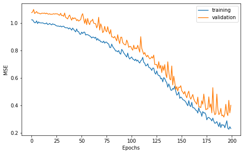
We can do a vizualisation of our learning curves to make sure the training and validation loss decrease correctly.
[9]:
width = 8
height = width/1.618
plt.figure(figsize=(width, height))

plt.plot(history["loss"], label="training")
plt.plot(history["val_loss"], label="validation")

plt.xlabel("Epochs")
plt.ylabel("MSE")

plt.legend()

plt.show()
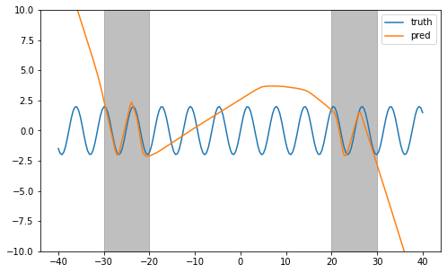
Also, let us look at the prediction on the test set after reversing the scaling of predicted variables.
[10]:
pred_s_ty = model(s_tx)
pred_ty = scaler_y.inverse_transform(pred_s_ty)

width = 8
height = width/1.618
plt.figure(figsize=(width, height))

plt.plot(tx, ty, label="truth")
plt.plot(tx, pred_ty, label="pred")

y_lim = 10
plt.fill_between([-30, -20], [-y_lim, -y_lim], [y_lim, y_lim], color="grey", alpha=0.5)
plt.fill_between([20, 30], [-y_lim, -y_lim], [y_lim, y_lim], color="grey", alpha=0.5)

plt.legend()
plt.ylim(-y_lim, y_lim)

plt.show()
3.6. Define the Neural Architecture Search Space#
The neural architecture search space is composed of discrete decision variables. For each decision variable we choose among a list of possible operation to perform (e.g., fully connected, ReLU). To define this search space, it is necessary to use two classes:
KSearchSpace(for Keras Search Space): represents a directed acyclic graph (DAG) in which each node represents a chosen operation. It represents the possible neural networks that can be created.SpaceFactory: is a utilitiy class used to pack the logic of a search space definition and share it with others.
Then, inside a KSearchSpace we will have two types of nodes: * VariableNode: corresponds to discrete decision variables and are used to define a list of possible operation. * ConstantNode: corresponds to fixed operation in the search space (e.g., input/outputs)
Finally, it is possible to reuse any tf.keras.layers to define a KSearchSpace. However, it is important to wrap each layer in an operation to perform a lazy memory allocation of tensors.
[11]:
import collections

from deephyper.nas import KSearchSpace

# Decision variables are represented by nodes in a graph
from deephyper.nas.node import ConstantNode, VariableNode

# The "operation" creates a wrapper around Keras layers avoid allocating
# memory each time a new layer is defined in the search space
# For Skip/Residual connections we use "Zero", "Connect" and "AddByProjecting"
from deephyper.nas.operation import operation, Zero, Connect, AddByProjecting, Identity

Dense = operation(tf.keras.layers.Dense)

# Possible activation functions
ACTIVATIONS = [
    tf.keras.activations.elu,
    tf.keras.activations.gelu,
    tf.keras.activations.hard_sigmoid,
    tf.keras.activations.linear,
    tf.keras.activations.relu,
    tf.keras.activations.selu,
    tf.keras.activations.sigmoid,
    tf.keras.activations.softplus,
    tf.keras.activations.softsign,
    tf.keras.activations.swish,
    tf.keras.activations.tanh,
]
We implement the constructor __init__ and build method of the RegressionSpace a subclass of KSearchSpace. The __init__ method interface is:
def __init__(self, input_shape, output_shape, **kwargs):
    ...
for the build method the interface is:
def build(self):
    ...
    return self
where: * input_shape corresponds to a tuple or a list of tuple indicating the shapes of inputs tensors. * output_shape corresponds to the same but of output_tensors. * **kwargs denotes that any other key word argument can be defined by the user.
[12]:
class RegressionSpace(KSearchSpace):

    def __init__(self, input_shape, output_shape, seed=None, num_layers=3):
        super().__init__(input_shape, output_shape, seed=seed)

        self.num_layers = 3

    def build(self):

        # After creating a KSearchSpace nodes corresponds to the inputs are directly accessible
        out_sub_graph = self.build_sub_graph(self.input_nodes[0], self.num_layers)

        output = ConstantNode(op=Dense(self.output_shape[0]))
        self.connect(out_sub_graph, output)

        return self

    def build_sub_graph(self, input_node, num_layers=3):


        # Look over skip connections within a range of the 3 previous nodes
        anchor_points = collections.deque([input_node], maxlen=3)

        prev_node = input_node

        for _ in range(num_layers):

            # Create a variable node to list possible "Dense" layers
            dense = VariableNode()

            # Add the possible operations to the dense node
            self.add_dense_to_(dense)

            # Connect the previous node to the dense node
            self.connect(prev_node, dense)

            # Create a constant node to merge all input connections
            merge = ConstantNode()
            merge.set_op(
                AddByProjecting(self, [dense], activation="relu")
            )

            for node in anchor_points:

                # Create a variable node for each possible connection
                skipco = VariableNode()

                skipco.add_op(Zero()) # corresponds to no connection
                skipco.add_op(Connect(self, node)) # corresponds to (node => skipco)

                # Connect the (skipco => merge)
                self.connect(skipco, merge)


            # ! for next iter
            prev_node = merge
            anchor_points.append(prev_node)

        return prev_node

    def add_dense_to_(self, node):

        # We add the "Identity" operation to allow the choice "doing nothing"
        node.add_op(Identity())

        step = 16
        for units in range(step, step * 16 + 1, step):
            for activation in ACTIVATIONS:
                node.add_op(Dense(units=units, activation=activation))
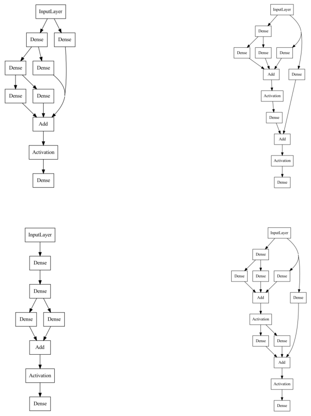
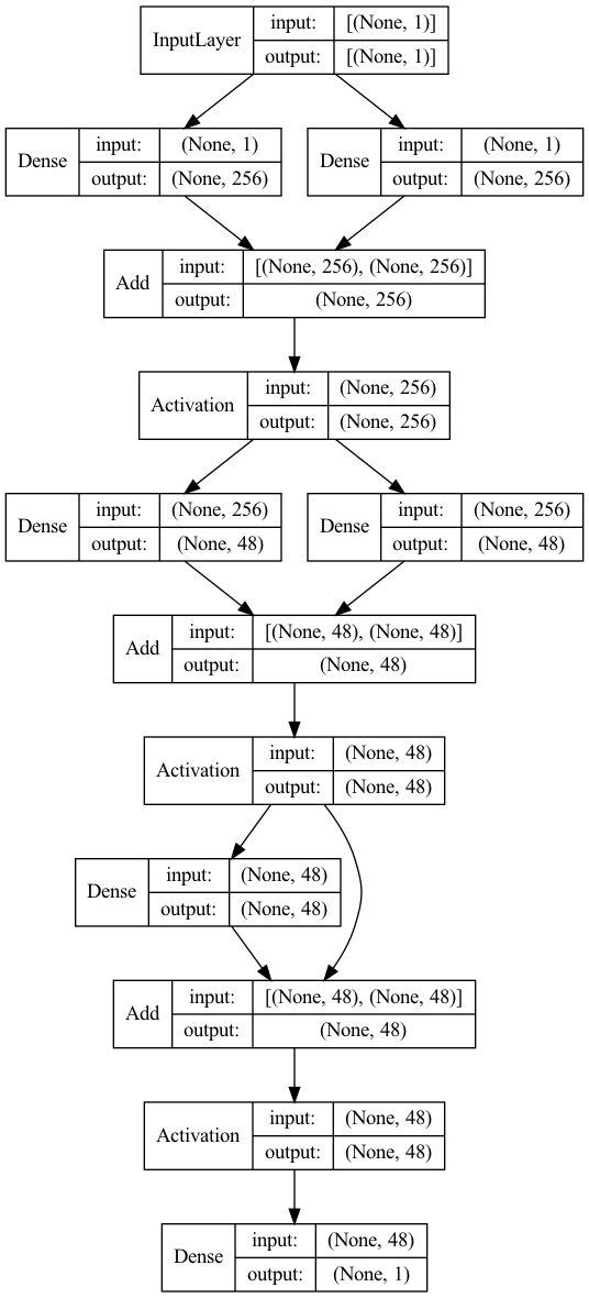
Let us visualize a few randomly sampled neural architecture from this search space.
[13]:
import matplotlib.image as mpimg
from tensorflow.keras.utils import plot_model

shapes = dict(input_shape=(1,), output_shape=(1,))
space = RegressionSpace(**shapes).build()


images = []
plt.figure(figsize=(15,15))
for i in range(4):

    model = space.sample()
    plt.subplot(2,2,i+1)
    plot_model(model, "random_model.png", show_shapes=False, show_layer_names=False)
    image = mpimg.imread("random_model.png")
    plt.imshow(image)
    plt.axis('off')

plt.show()
3.7. Define the Neural Architecture Optimization Problem#
In order to define a neural architecture search problem we have to use the NaProblem class. This class gives access to different method for the user to customize the training settings of neural networks.
[14]:
from deephyper.problem import NaProblem


def stdscaler():
    return StandardScaler()


problem = NaProblem()

# Bind a function which returns (train_input, train_output), (valid_input, valid_output)
problem.load_data(load_data_train_valid)

# Bind a function which return a scikit-learn preprocessor (with fit, fit_transform, inv_transform...etc)
problem.preprocessing(stdscaler)

# Bind a function which returns a search space and give some arguments for the `build` method
problem.search_space(RegressionSpace, num_layers=3)

# Define a set of fixed hyperparameters for all trained neural networks
problem.hyperparameters(
    batch_size=4,
    learning_rate=1e-3,
    optimizer="adam",
    epsilon=1e-7,
    num_epochs=200,
    callbacks=dict(
        EarlyStopping=dict(monitor="val_loss", mode="min", verbose=0, patience=30)
    ),
)

# Define the loss to minimize
problem.loss("mse")

# Define complementary metrics
problem.metrics([])

# Define the maximized objective. Here we take the negative of the validation loss.
problem.objective("-val_loss")

problem
[14]:
Problem is:
    - search space   : __main__.RegressionSpace
    - data loading   : __main__.load_data_train_valid
    - preprocessing  : __main__.stdscaler
    - hyperparameters:
        * verbose: 0
        * batch_size: 4
        * learning_rate: 0.001
        * optimizer: adam
        * num_epochs: 200
        * callbacks: {'EarlyStopping': {'monitor': 'val_loss', 'mode': 'min', 'verbose': 0, 'patience': 30}}
    - loss           : mse
    - metrics        :
    - objective      : -val_loss
Tip
Adding an EarlyStopping(...) callback is a good idea to stop the training of your model as soon as it stops to improve.
...
EarlyStopping=dict(monitor="val_loss", mode="min", verbose=0, patience=30)
...
3.8. Define the Evaluator Object#
The Evaluator object is responsible of defining the backend used to distribute the function evaluation in DeepHyper.
[15]:
from deephyper.evaluator import Evaluator
from deephyper.evaluator.callback import TqdmCallback


def get_evaluator(run_function):

    # Default arguments for Ray: 1 worker and 1 worker per evaluation
    method_kwargs = {
        "num_cpus": 1,
        "num_cpus_per_task": 1,
        "callbacks": [TqdmCallback()] # To interactively follow the finished evaluations,
    }

    # If GPU devices are detected then it will create 'n_gpus' workers
    # and use 1 worker for each evaluation
    if is_gpu_available:
        method_kwargs["num_cpus"] = n_gpus
        method_kwargs["num_gpus"] = n_gpus
        method_kwargs["num_cpus_per_task"] = 1
        method_kwargs["num_gpus_per_task"] = 1

    evaluator = Evaluator.create(
        run_function,
        method="ray",
        method_kwargs=method_kwargs
    )
    print(f"Created new evaluator with {evaluator.num_workers} worker{'s' if evaluator.num_workers > 1 else ''} and config: {method_kwargs}", )

    return evaluator
For neural architecture search a standard training pipeline is provided by the run_base_trainer function from the deephyper.nas.run module.
[16]:
from deephyper.nas.run import run_base_trainer
3.9. Define and Run the Neural Architecture Search#
All search algorithms follow a similar interface. A problem and evaluator object has to be provided to the search then the search can be executed through the search(max_evals, timeout) method.
[17]:
results = {} # used to store the results of different search algorithms
max_evals = 10 # maximum number of iteratins for all searches
[18]:
from deephyper.search.nas import Random

random_search = Random(problem, get_evaluator(run_base_trainer), log_dir="random_search")

results["random"] = random_search.search(max_evals=max_evals)
/Users/romainegele/Documents/Argonne/deephyper/deephyper/evaluator/_evaluator.py:99: UserWarning: Applying nest-asyncio patch for IPython Shell!
  warnings.warn(
Created new evaluator with 4 workers and config: {'num_cpus': 1, 'num_cpus_per_task': 1, 'callbacks': [<deephyper.evaluator.callback.TqdmCallback object at 0x3453184c0>]}
By default, the RegularizedEvolution has a population size of 100 therefore, it will start optimizing only after 100 evaluations.
[19]:
from deephyper.search.nas import RegularizedEvolution

regevo_search = RegularizedEvolution(problem, get_evaluator(run_base_trainer), log_dir="regevo_search")

results["regevo"] = regevo_search.search(max_evals=max_evals)
/Users/romainegele/Documents/Argonne/deephyper/deephyper/evaluator/_evaluator.py:99: UserWarning: Applying nest-asyncio patch for IPython Shell!
  warnings.warn(
Created new evaluator with 4 workers and config: {'num_cpus': 1, 'num_cpus_per_task': 1, 'callbacks': [<deephyper.evaluator.callback.TqdmCallback object at 0x3469c0550>]}
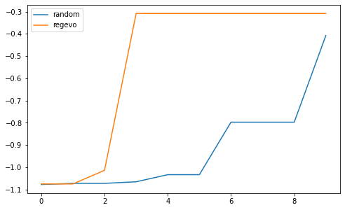
We can now compare the search trajectories for different algorithms.
[20]:
def max_score(l):
    r = [l[0]]
    for el in l[1:]:
        r.append(max(r[-1], el))
    return r

width = 8
height = width/1.618
plt.figure(figsize=(width, height))

for k, result in results.items():
    plt.plot(max_score(results[k].objective), label=k)

plt.legend()

plt.show()
If we look at the dataframe of results for each search we will find it slightly different than the one of hyperparameter search. A new column arch_seq corresponds to an embedding for each evaluated architecture. Each integer of an arch_seq list corresponds to the choice of a VariableNode in our KSearchSpace.
[21]:
results["random"]
[21]:
| arch_seq | job_id | objective | timestamp_submit | timestamp_gather | |
|---|---|---|---|---|---|
| 0 | [46, 0, 156, 0, 0, 44, 0, 1, 0] | 4 | -1.077856 | 0.007198 | 4.211616 |
| 1 | [53, 0, 133, 0, 0, 52, 0, 0, 0] | 3 | -1.072681 | 0.007162 | 4.243041 |
| 2 | [62, 0, 112, 1, 1, 115, 1, 1, 1] | 2 | -1.078561 | 0.007126 | 4.252246 |
| 3 | [71, 1, 22, 1, 1, 161, 1, 0, 0] | 5 | -1.065605 | 4.234786 | 6.294323 |
| 4 | [107, 1, 27, 1, 0, 68, 0, 0, 0] | 6 | -1.033612 | 4.244888 | 8.575346 |
| 5 | [19, 1, 161, 1, 1, 132, 1, 1, 1] | 7 | -1.069055 | 4.253639 | 9.027878 |
| 6 | [166, 1, 19, 1, 0, 40, 0, 1, 0] | 1 | -0.797477 | 0.007086 | 9.302246 |
| 7 | [164, 0, 30, 0, 0, 121, 1, 1, 0] | 9 | -1.097940 | 8.577058 | 10.901906 |
| 8 | [17, 0, 64, 1, 0, 121, 1, 0, 1] | 10 | -1.134835 | 9.029494 | 13.366727 |
| 9 | [175, 1, 26, 0, 1, 29, 0, 0, 1] | 8 | -0.407744 | 6.296113 | 13.541472 |
Let us visualize the best architecture found:
[22]:
i_max = results["random"].objective.argmax()
best_score = results["random"].iloc[i_max].objective
best_arch_seq = json.loads(results["random"].iloc[i_max].arch_seq)

best_model = space.sample(best_arch_seq)
plot_model(best_model, show_shapes=True, show_layer_names=False)
[22]:
3.10. Adding Uncertainty Quantification to the Baseline Neural Network#
To add uncertainty estimates we use the Tensorflow Probability library which is fully compatible with the neural architecture search API because it is accessible through Keras layers.
[23]:
import tensorflow_probability as tfp
tfd = tfp.distributions
Then, instead of minimising the mean squared error we will minimize the negative log-likelihood baed on the learned probability distribution \(p(y|\mathbf{x};\theta)\) where \(\theta\) represents a neural network (architecture, training hyperparameters, weights).
[24]:
def nll(y, rv_y):
    """Negative log likelihood for Tensorflow probability.

    Args:
        y: true data.
        rv_y: learned (predicted) probability distribution.
    """
    return -rv_y.log_prob(y)
[25]:
input_ = tf.keras.layers.Input(shape=(1,))
out = tf.keras.layers.Dense(200, activation="relu")(input_)
out = tf.keras.layers.Dense(200, activation="relu")(out)

# For each predicted variable (1) we need the mean and variance estimate
out = tf.keras.layers.Dense(1*2)(out)

# We feed these estimates to output a Normal distribution for each predicted variable
output = tfp.layers.DistributionLambda(
            lambda t: tfd.Normal(
                loc=t[..., :1],
                scale=1e-3 + tf.math.softplus(0.05 * t[..., 1:]), # positive constraint on the standard dev.
            )
        )(out)

model_uq = tf.keras.Model(input_, output)

optimizer = tf.keras.optimizers.Adam(learning_rate=1e-3)
model_uq.compile(optimizer, loss=nll)

history = model_uq.fit(s_x, s_y, epochs=200, batch_size=4, validation_data=(s_vx, s_vy), verbose=1)
Epoch 1/200
 1/67 [..............................] - ETA: 8s - loss: 1.2174
2022-06-08 11:33:24.578012: W tensorflow/python/util/util.cc:348] Sets are not currently considered sequences, but this may change in the future, so consider avoiding using them.
67/67 [==============================] - 0s 1ms/step - loss: 1.6107 - val_loss: 1.6747
Epoch 2/200
67/67 [==============================] - 0s 646us/step - loss: 1.5902 - val_loss: 1.6257
Epoch 3/200
67/67 [==============================] - 0s 635us/step - loss: 1.5455 - val_loss: 1.6290
Epoch 4/200
67/67 [==============================] - 0s 624us/step - loss: 1.5151 - val_loss: 1.5265
Epoch 5/200
67/67 [==============================] - 0s 618us/step - loss: 1.4994 - val_loss: 1.4860
Epoch 6/200
67/67 [==============================] - 0s 621us/step - loss: 1.4405 - val_loss: 1.4940
Epoch 7/200
67/67 [==============================] - 0s 619us/step - loss: 1.4344 - val_loss: 1.4571
Epoch 8/200
67/67 [==============================] - 0s 607us/step - loss: 1.4260 - val_loss: 1.4532
Epoch 9/200
67/67 [==============================] - 0s 618us/step - loss: 1.4328 - val_loss: 1.4545
Epoch 10/200
67/67 [==============================] - 0s 616us/step - loss: 1.4340 - val_loss: 1.4684
Epoch 11/200
67/67 [==============================] - 0s 603us/step - loss: 1.4314 - val_loss: 1.4744
Epoch 12/200
67/67 [==============================] - 0s 610us/step - loss: 1.4317 - val_loss: 1.4697
Epoch 13/200
67/67 [==============================] - 0s 610us/step - loss: 1.4317 - val_loss: 1.4557
Epoch 14/200
67/67 [==============================] - 0s 618us/step - loss: 1.4285 - val_loss: 1.4514
Epoch 15/200
67/67 [==============================] - 0s 613us/step - loss: 1.4255 - val_loss: 1.4481
Epoch 16/200
67/67 [==============================] - 0s 663us/step - loss: 1.4252 - val_loss: 1.4934
Epoch 17/200
67/67 [==============================] - 0s 690us/step - loss: 1.4270 - val_loss: 1.4569
Epoch 18/200
67/67 [==============================] - 0s 626us/step - loss: 1.4308 - val_loss: 1.4677
Epoch 19/200
67/67 [==============================] - 0s 605us/step - loss: 1.4255 - val_loss: 1.4575
Epoch 20/200
67/67 [==============================] - 0s 612us/step - loss: 1.4224 - val_loss: 1.4590
Epoch 21/200
67/67 [==============================] - 0s 616us/step - loss: 1.4223 - val_loss: 1.4629
Epoch 22/200
67/67 [==============================] - 0s 616us/step - loss: 1.4240 - val_loss: 1.4692
Epoch 23/200
67/67 [==============================] - 0s 607us/step - loss: 1.4280 - val_loss: 1.4493
Epoch 24/200
67/67 [==============================] - 0s 615us/step - loss: 1.4211 - val_loss: 1.4660
Epoch 25/200
67/67 [==============================] - 0s 619us/step - loss: 1.4216 - val_loss: 1.4586
Epoch 26/200
67/67 [==============================] - 0s 655us/step - loss: 1.4135 - val_loss: 1.4496
Epoch 27/200
67/67 [==============================] - 0s 610us/step - loss: 1.4185 - val_loss: 1.4622
Epoch 28/200
67/67 [==============================] - 0s 606us/step - loss: 1.4142 - val_loss: 1.4607
Epoch 29/200
67/67 [==============================] - 0s 603us/step - loss: 1.4153 - val_loss: 1.4598
Epoch 30/200
67/67 [==============================] - 0s 617us/step - loss: 1.4188 - val_loss: 1.4671
Epoch 31/200
67/67 [==============================] - 0s 624us/step - loss: 1.4154 - val_loss: 1.4498
Epoch 32/200
67/67 [==============================] - 0s 614us/step - loss: 1.4172 - val_loss: 1.4441
Epoch 33/200
67/67 [==============================] - 0s 618us/step - loss: 1.4139 - val_loss: 1.4554
Epoch 34/200
67/67 [==============================] - 0s 619us/step - loss: 1.4174 - val_loss: 1.4469
Epoch 35/200
67/67 [==============================] - 0s 604us/step - loss: 1.4139 - val_loss: 1.4638
Epoch 36/200
67/67 [==============================] - 0s 619us/step - loss: 1.4212 - val_loss: 1.4540
Epoch 37/200
67/67 [==============================] - 0s 603us/step - loss: 1.4085 - val_loss: 1.4632
Epoch 38/200
67/67 [==============================] - 0s 621us/step - loss: 1.4106 - val_loss: 1.4531
Epoch 39/200
67/67 [==============================] - 0s 622us/step - loss: 1.4136 - val_loss: 1.4556
Epoch 40/200
67/67 [==============================] - 0s 620us/step - loss: 1.4106 - val_loss: 1.4433
Epoch 41/200
67/67 [==============================] - 0s 602us/step - loss: 1.4139 - val_loss: 1.4550
Epoch 42/200
67/67 [==============================] - 0s 616us/step - loss: 1.4115 - val_loss: 1.4526
Epoch 43/200
67/67 [==============================] - 0s 584us/step - loss: 1.4131 - val_loss: 1.4553
Epoch 44/200
67/67 [==============================] - 0s 601us/step - loss: 1.4100 - val_loss: 1.4651
Epoch 45/200
67/67 [==============================] - 0s 612us/step - loss: 1.4085 - val_loss: 1.4433
Epoch 46/200
67/67 [==============================] - 0s 635us/step - loss: 1.4058 - val_loss: 1.4475
Epoch 47/200
67/67 [==============================] - 0s 645us/step - loss: 1.4087 - val_loss: 1.4474
Epoch 48/200
67/67 [==============================] - 0s 618us/step - loss: 1.4110 - val_loss: 1.4424
Epoch 49/200
67/67 [==============================] - 0s 616us/step - loss: 1.4050 - val_loss: 1.4419
Epoch 50/200
67/67 [==============================] - 0s 828us/step - loss: 1.4043 - val_loss: 1.4776
Epoch 51/200
67/67 [==============================] - 0s 600us/step - loss: 1.4093 - val_loss: 1.4692
Epoch 52/200
67/67 [==============================] - 0s 627us/step - loss: 1.4119 - val_loss: 1.4483
Epoch 53/200
67/67 [==============================] - 0s 592us/step - loss: 1.4039 - val_loss: 1.4913
Epoch 54/200
67/67 [==============================] - 0s 600us/step - loss: 1.4092 - val_loss: 1.4437
Epoch 55/200
67/67 [==============================] - 0s 617us/step - loss: 1.4110 - val_loss: 1.4437
Epoch 56/200
67/67 [==============================] - 0s 603us/step - loss: 1.4053 - val_loss: 1.4599
Epoch 57/200
67/67 [==============================] - 0s 627us/step - loss: 1.3927 - val_loss: 1.4480
Epoch 58/200
67/67 [==============================] - 0s 603us/step - loss: 1.4035 - val_loss: 1.4448
Epoch 59/200
67/67 [==============================] - 0s 608us/step - loss: 1.3986 - val_loss: 1.4409
Epoch 60/200
67/67 [==============================] - 0s 613us/step - loss: 1.4011 - val_loss: 1.4497
Epoch 61/200
67/67 [==============================] - 0s 639us/step - loss: 1.3996 - val_loss: 1.4382
Epoch 62/200
67/67 [==============================] - 0s 629us/step - loss: 1.4027 - val_loss: 1.4406
Epoch 63/200
67/67 [==============================] - 0s 602us/step - loss: 1.3986 - val_loss: 1.4650
Epoch 64/200
67/67 [==============================] - 0s 613us/step - loss: 1.3941 - val_loss: 1.4359
Epoch 65/200
67/67 [==============================] - 0s 602us/step - loss: 1.4061 - val_loss: 1.4366
Epoch 66/200
67/67 [==============================] - 0s 597us/step - loss: 1.4079 - val_loss: 1.4450
Epoch 67/200
67/67 [==============================] - 0s 617us/step - loss: 1.3928 - val_loss: 1.4396
Epoch 68/200
67/67 [==============================] - 0s 604us/step - loss: 1.3949 - val_loss: 1.4348
Epoch 69/200
67/67 [==============================] - 0s 609us/step - loss: 1.3902 - val_loss: 1.4558
Epoch 70/200
67/67 [==============================] - 0s 604us/step - loss: 1.3957 - val_loss: 1.4369
Epoch 71/200
67/67 [==============================] - 0s 609us/step - loss: 1.3981 - val_loss: 1.4495
Epoch 72/200
67/67 [==============================] - 0s 616us/step - loss: 1.3966 - val_loss: 1.4285
Epoch 73/200
67/67 [==============================] - 0s 617us/step - loss: 1.3857 - val_loss: 1.4354
Epoch 74/200
67/67 [==============================] - 0s 610us/step - loss: 1.3900 - val_loss: 1.4284
Epoch 75/200
67/67 [==============================] - 0s 617us/step - loss: 1.3782 - val_loss: 1.4454
Epoch 76/200
67/67 [==============================] - 0s 617us/step - loss: 1.3856 - val_loss: 1.4287
Epoch 77/200
67/67 [==============================] - 0s 626us/step - loss: 1.3798 - val_loss: 1.4328
Epoch 78/200
67/67 [==============================] - 0s 603us/step - loss: 1.3780 - val_loss: 1.4219
Epoch 79/200
67/67 [==============================] - 0s 627us/step - loss: 1.3737 - val_loss: 1.4278
Epoch 80/200
67/67 [==============================] - 0s 594us/step - loss: 1.3655 - val_loss: 1.4188
Epoch 81/200
67/67 [==============================] - 0s 610us/step - loss: 1.3579 - val_loss: 1.4404
Epoch 82/200
67/67 [==============================] - 0s 600us/step - loss: 1.3737 - val_loss: 1.4367
Epoch 83/200
67/67 [==============================] - 0s 618us/step - loss: 1.3727 - val_loss: 1.4446
Epoch 84/200
67/67 [==============================] - 0s 617us/step - loss: 1.3702 - val_loss: 1.4129
Epoch 85/200
67/67 [==============================] - 0s 609us/step - loss: 1.3648 - val_loss: 1.4146
Epoch 86/200
67/67 [==============================] - 0s 604us/step - loss: 1.3655 - val_loss: 1.4285
Epoch 87/200
67/67 [==============================] - 0s 621us/step - loss: 1.3706 - val_loss: 1.4126
Epoch 88/200
67/67 [==============================] - 0s 611us/step - loss: 1.3643 - val_loss: 1.4194
Epoch 89/200
67/67 [==============================] - 0s 606us/step - loss: 1.3596 - val_loss: 1.4144
Epoch 90/200
67/67 [==============================] - 0s 601us/step - loss: 1.3572 - val_loss: 1.4106
Epoch 91/200
67/67 [==============================] - 0s 621us/step - loss: 1.3497 - val_loss: 1.4179
Epoch 92/200
67/67 [==============================] - 0s 595us/step - loss: 1.3605 - val_loss: 1.4135
Epoch 93/200
67/67 [==============================] - 0s 620us/step - loss: 1.3469 - val_loss: 1.4164
Epoch 94/200
67/67 [==============================] - 0s 622us/step - loss: 1.3448 - val_loss: 1.4624
Epoch 95/200
67/67 [==============================] - 0s 612us/step - loss: 1.3431 - val_loss: 1.4051
Epoch 96/200
67/67 [==============================] - 0s 612us/step - loss: 1.3353 - val_loss: 1.4127
Epoch 97/200
67/67 [==============================] - 0s 605us/step - loss: 1.3394 - val_loss: 1.4094
Epoch 98/200
67/67 [==============================] - 0s 622us/step - loss: 1.3486 - val_loss: 1.3978
Epoch 99/200
67/67 [==============================] - 0s 614us/step - loss: 1.3490 - val_loss: 1.3896
Epoch 100/200
67/67 [==============================] - 0s 612us/step - loss: 1.3332 - val_loss: 1.4128
Epoch 101/200
67/67 [==============================] - 0s 622us/step - loss: 1.3326 - val_loss: 1.4218
Epoch 102/200
67/67 [==============================] - 0s 613us/step - loss: 1.3285 - val_loss: 1.4253
Epoch 103/200
67/67 [==============================] - 0s 613us/step - loss: 1.3712 - val_loss: 1.3852
Epoch 104/200
67/67 [==============================] - 0s 614us/step - loss: 1.3491 - val_loss: 1.3914
Epoch 105/200
67/67 [==============================] - 0s 600us/step - loss: 1.3246 - val_loss: 1.3953
Epoch 106/200
67/67 [==============================] - 0s 619us/step - loss: 1.3167 - val_loss: 1.3745
Epoch 107/200
67/67 [==============================] - 0s 615us/step - loss: 1.3143 - val_loss: 1.3770
Epoch 108/200
67/67 [==============================] - 0s 609us/step - loss: 1.3161 - val_loss: 1.3864
Epoch 109/200
67/67 [==============================] - 0s 631us/step - loss: 1.3044 - val_loss: 1.3644
Epoch 110/200
67/67 [==============================] - 0s 603us/step - loss: 1.2976 - val_loss: 1.3662
Epoch 111/200
67/67 [==============================] - 0s 619us/step - loss: 1.3263 - val_loss: 1.3881
Epoch 112/200
67/67 [==============================] - 0s 610us/step - loss: 1.3296 - val_loss: 1.3708
Epoch 113/200
67/67 [==============================] - 0s 623us/step - loss: 1.2924 - val_loss: 1.3549
Epoch 114/200
67/67 [==============================] - 0s 606us/step - loss: 1.2924 - val_loss: 1.3609
Epoch 115/200
67/67 [==============================] - 0s 624us/step - loss: 1.2882 - val_loss: 1.3621
Epoch 116/200
67/67 [==============================] - 0s 605us/step - loss: 1.2843 - val_loss: 1.3656
Epoch 117/200
67/67 [==============================] - 0s 624us/step - loss: 1.2717 - val_loss: 1.3360
Epoch 118/200
67/67 [==============================] - 0s 601us/step - loss: 1.2703 - val_loss: 1.3440
Epoch 119/200
67/67 [==============================] - 0s 609us/step - loss: 1.2827 - val_loss: 1.3278
Epoch 120/200
67/67 [==============================] - 0s 611us/step - loss: 1.2577 - val_loss: 1.3147
Epoch 121/200
67/67 [==============================] - 0s 614us/step - loss: 1.2600 - val_loss: 1.5124
Epoch 122/200
67/67 [==============================] - 0s 622us/step - loss: 1.2616 - val_loss: 1.3171
Epoch 123/200
67/67 [==============================] - 0s 621us/step - loss: 1.2310 - val_loss: 1.3457
Epoch 124/200
67/67 [==============================] - 0s 621us/step - loss: 1.2484 - val_loss: 1.2970
Epoch 125/200
67/67 [==============================] - 0s 619us/step - loss: 1.2351 - val_loss: 1.3229
Epoch 126/200
67/67 [==============================] - 0s 606us/step - loss: 1.2294 - val_loss: 1.2987
Epoch 127/200
67/67 [==============================] - 0s 622us/step - loss: 1.2096 - val_loss: 1.3402
Epoch 128/200
67/67 [==============================] - 0s 607us/step - loss: 1.2136 - val_loss: 1.3656
Epoch 129/200
67/67 [==============================] - 0s 630us/step - loss: 1.2462 - val_loss: 1.3228
Epoch 130/200
67/67 [==============================] - 0s 611us/step - loss: 1.2008 - val_loss: 1.2843
Epoch 131/200
67/67 [==============================] - 0s 606us/step - loss: 1.1903 - val_loss: 1.2580
Epoch 132/200
67/67 [==============================] - 0s 609us/step - loss: 1.2018 - val_loss: 1.2824
Epoch 133/200
67/67 [==============================] - 0s 609us/step - loss: 1.1724 - val_loss: 1.2708
Epoch 134/200
67/67 [==============================] - 0s 606us/step - loss: 1.1700 - val_loss: 1.2727
Epoch 135/200
67/67 [==============================] - 0s 615us/step - loss: 1.1908 - val_loss: 1.2403
Epoch 136/200
67/67 [==============================] - 0s 615us/step - loss: 1.1559 - val_loss: 1.3048
Epoch 137/200
67/67 [==============================] - 0s 609us/step - loss: 1.1890 - val_loss: 1.2424
Epoch 138/200
67/67 [==============================] - 0s 612us/step - loss: 1.1697 - val_loss: 1.2306
Epoch 139/200
67/67 [==============================] - 0s 617us/step - loss: 1.1727 - val_loss: 1.3151
Epoch 140/200
67/67 [==============================] - 0s 615us/step - loss: 1.1459 - val_loss: 1.2019
Epoch 141/200
67/67 [==============================] - 0s 598us/step - loss: 1.1379 - val_loss: 1.2438
Epoch 142/200
67/67 [==============================] - 0s 615us/step - loss: 1.1456 - val_loss: 1.3272
Epoch 143/200
67/67 [==============================] - 0s 618us/step - loss: 1.1496 - val_loss: 1.2206
Epoch 144/200
67/67 [==============================] - 0s 620us/step - loss: 1.1345 - val_loss: 1.2179
Epoch 145/200
67/67 [==============================] - 0s 612us/step - loss: 1.1874 - val_loss: 1.1936
Epoch 146/200
67/67 [==============================] - 0s 617us/step - loss: 1.1108 - val_loss: 1.3553
Epoch 147/200
67/67 [==============================] - 0s 606us/step - loss: 1.2347 - val_loss: 1.3395
Epoch 148/200
67/67 [==============================] - 0s 607us/step - loss: 1.2345 - val_loss: 1.2146
Epoch 149/200
67/67 [==============================] - 0s 615us/step - loss: 1.0859 - val_loss: 1.1817
Epoch 150/200
67/67 [==============================] - 0s 617us/step - loss: 1.1205 - val_loss: 1.2697
Epoch 151/200
67/67 [==============================] - 0s 615us/step - loss: 1.1634 - val_loss: 1.2113
Epoch 152/200
67/67 [==============================] - 0s 612us/step - loss: 1.0946 - val_loss: 1.1572
Epoch 153/200
67/67 [==============================] - 0s 615us/step - loss: 1.0643 - val_loss: 1.1665
Epoch 154/200
67/67 [==============================] - 0s 627us/step - loss: 1.0984 - val_loss: 1.1411
Epoch 155/200
67/67 [==============================] - 0s 609us/step - loss: 1.0409 - val_loss: 1.1030
Epoch 156/200
67/67 [==============================] - 0s 638us/step - loss: 1.0751 - val_loss: 1.1155
Epoch 157/200
67/67 [==============================] - 0s 604us/step - loss: 1.0108 - val_loss: 1.1772
Epoch 158/200
67/67 [==============================] - 0s 613us/step - loss: 1.1279 - val_loss: 1.1156
Epoch 159/200
67/67 [==============================] - 0s 600us/step - loss: 1.0118 - val_loss: 1.2895
Epoch 160/200
67/67 [==============================] - 0s 614us/step - loss: 1.0863 - val_loss: 1.1346
Epoch 161/200
67/67 [==============================] - 0s 607us/step - loss: 1.0203 - val_loss: 1.0433
Epoch 162/200
67/67 [==============================] - 0s 616us/step - loss: 0.9536 - val_loss: 1.0468
Epoch 163/200
67/67 [==============================] - 0s 614us/step - loss: 0.9703 - val_loss: 1.0567
Epoch 164/200
67/67 [==============================] - 0s 617us/step - loss: 0.9687 - val_loss: 1.0309
Epoch 165/200
67/67 [==============================] - 0s 601us/step - loss: 0.9433 - val_loss: 0.9975
Epoch 166/200
67/67 [==============================] - 0s 613us/step - loss: 0.9616 - val_loss: 0.9652
Epoch 167/200
67/67 [==============================] - 0s 606us/step - loss: 0.8975 - val_loss: 0.9744
Epoch 168/200
67/67 [==============================] - 0s 612us/step - loss: 0.8896 - val_loss: 0.9621
Epoch 169/200
67/67 [==============================] - 0s 607us/step - loss: 0.8824 - val_loss: 1.0194
Epoch 170/200
67/67 [==============================] - 0s 624us/step - loss: 0.9065 - val_loss: 0.9161
Epoch 171/200
67/67 [==============================] - 0s 602us/step - loss: 0.8750 - val_loss: 0.9509
Epoch 172/200
67/67 [==============================] - 0s 616us/step - loss: 0.8899 - val_loss: 0.9551
Epoch 173/200
67/67 [==============================] - 0s 614us/step - loss: 0.9543 - val_loss: 0.9048
Epoch 174/200
67/67 [==============================] - 0s 610us/step - loss: 0.8608 - val_loss: 0.8735
Epoch 175/200
67/67 [==============================] - 0s 605us/step - loss: 0.8347 - val_loss: 0.9168
Epoch 176/200
67/67 [==============================] - 0s 623us/step - loss: 0.8830 - val_loss: 0.9163
Epoch 177/200
67/67 [==============================] - 0s 602us/step - loss: 0.9072 - val_loss: 0.9237
Epoch 178/200
67/67 [==============================] - 0s 630us/step - loss: 0.8289 - val_loss: 0.9404
Epoch 179/200
67/67 [==============================] - 0s 599us/step - loss: 0.8229 - val_loss: 0.9293
Epoch 180/200
67/67 [==============================] - 0s 625us/step - loss: 0.8387 - val_loss: 0.8966
Epoch 181/200
67/67 [==============================] - 0s 612us/step - loss: 0.7761 - val_loss: 0.8522
Epoch 182/200
67/67 [==============================] - 0s 618us/step - loss: 0.8652 - val_loss: 1.2645
Epoch 183/200
67/67 [==============================] - 0s 611us/step - loss: 0.8201 - val_loss: 0.8661
Epoch 184/200
67/67 [==============================] - 0s 629us/step - loss: 0.8743 - val_loss: 0.9136
Epoch 185/200
67/67 [==============================] - 0s 611us/step - loss: 0.7791 - val_loss: 0.8688
Epoch 186/200
67/67 [==============================] - 0s 623us/step - loss: 0.8164 - val_loss: 0.9601
Epoch 187/200
67/67 [==============================] - 0s 792us/step - loss: 0.8150 - val_loss: 0.8607
Epoch 188/200
67/67 [==============================] - 0s 626us/step - loss: 0.7764 - val_loss: 0.8476
Epoch 189/200
67/67 [==============================] - 0s 607us/step - loss: 0.7622 - val_loss: 0.8193
Epoch 190/200
67/67 [==============================] - 0s 611us/step - loss: 0.7697 - val_loss: 0.7979
Epoch 191/200
67/67 [==============================] - 0s 613us/step - loss: 0.8272 - val_loss: 0.8666
Epoch 192/200
67/67 [==============================] - 0s 605us/step - loss: 0.7263 - val_loss: 0.8312
Epoch 193/200
67/67 [==============================] - 0s 621us/step - loss: 0.7563 - val_loss: 0.8916
Epoch 194/200
67/67 [==============================] - 0s 616us/step - loss: 0.7682 - val_loss: 0.8703
Epoch 195/200
67/67 [==============================] - 0s 617us/step - loss: 0.7732 - val_loss: 0.8403
Epoch 196/200
67/67 [==============================] - 0s 606us/step - loss: 0.7330 - val_loss: 0.8595
Epoch 197/200
67/67 [==============================] - 0s 614us/step - loss: 0.7962 - val_loss: 0.8104
Epoch 198/200
67/67 [==============================] - 0s 622us/step - loss: 0.7321 - val_loss: 0.8577
Epoch 199/200
67/67 [==============================] - 0s 611us/step - loss: 0.7553 - val_loss: 0.8706
Epoch 200/200
67/67 [==============================] - 0s 625us/step - loss: 0.7440 - val_loss: 0.8125
[26]:
width = 8
height = width/1.618
plt.figure(figsize=(width, height))

plt.plot(history.history["loss"], label="training")
plt.plot(history.history["val_loss"], label="validation")

plt.xlabel("Epochs")
plt.ylabel("NLL")

plt.legend()

plt.show()
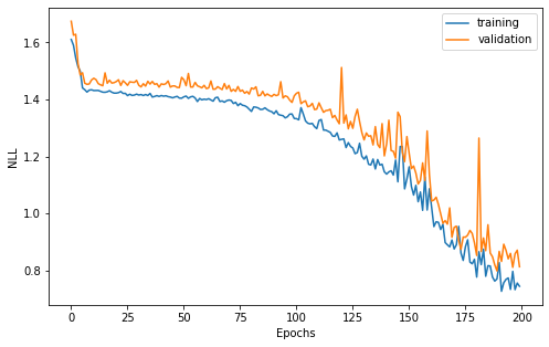
Let us visualize the learned uncertainty estimates.
[27]:
pred_s_ty = model_uq(s_tx)

pred_ty_mean = pred_s_ty.loc.numpy() + scaler_y.mean_
pred_ty_var = np.square(pred_s_ty.scale.numpy()) * scaler_y.var_

width = 8
height = width/1.618
plt.figure(figsize=(width, height))

plt.plot(tx, ty, label="truth")
plt.plot(tx, pred_ty_mean, label="$\mu$")
plt.fill_between(
    tx.reshape(-1),
    (pred_ty_mean - pred_ty_var).reshape(-1),
    (pred_ty_mean + pred_ty_var).reshape(-1),
    color="orange",
    alpha=0.5,
    label="$\sigma^2$"
)

y_lim = 10
plt.fill_between([-30, -20], [-y_lim, -y_lim], [y_lim, y_lim], color="grey", alpha=0.5)
plt.fill_between([20, 30], [-y_lim, -y_lim], [y_lim, y_lim], color="grey", alpha=0.5)

plt.legend()
plt.ylim(-y_lim, y_lim)

plt.show()
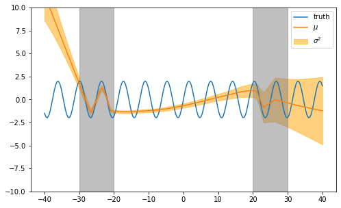
The learned mean estimates appears to be worse than when minimizing the mean squared error loss. Also, we can see than the variance estimate are not meaningful in areas missing data (white background) and do not learn properly the noise in are with data (grey background).
3.11. Ensemble of Neural Networks With Random Initialization#
The uncertainty estimate of a single neural network corresponds to aleatoric uncertainty (i.e., intrinsic noise of the data). To estimate the epistemic uncertainty, composed of estimation uncertainty (e.g., optimization algorithm) and model uncertainty (e.g., hypothesis space of models), we need to quantify the variation of predictions for different models and estimation. One of the most basic method to do it is to keep a fixed neural network architecture and training hyperparameters to then re-train it multiple times from different random weight initialization.
[28]:
def generate_model(model_id):

    # Model
    input_ = tf.keras.layers.Input(shape=(1,))
    out = tf.keras.layers.Dense(200, activation="relu")(input_)
    out = tf.keras.layers.Dense(200, activation="relu")(out)
    out = tf.keras.layers.Dense(2)(out) # 1 unit for the mean, 1 unit for the scale
    output = tfp.layers.DistributionLambda(
                lambda t: tfd.Normal(
                    loc=t[..., :1],
                    scale=1e-3 + tf.math.softplus(0.05 * t[..., 1:]),
                )
            )(out)
    model_uq = tf.keras.Model(input_, output)


    model_checkpoint_callback = tf.keras.callbacks.ModelCheckpoint(
        filepath=os.path.join("models_random_init", f"{model_id}.h5"),
        monitor='val_loss',
        verbose=0,
        save_best_only=True,
        save_weights_only=False,
        mode='min',
        save_freq='epoch'
    )

    optimizer = tf.keras.optimizers.Adam(learning_rate=1e-3)
    model_uq.compile(optimizer, loss=nll)

    history = model_uq.fit(s_x, s_y,
                           epochs=200,
                           batch_size=4,
                           validation_data=(s_vx, s_vy),
                           verbose=0,
                           callbacks=[model_checkpoint_callback]
                          ).history
    return history["val_loss"][-1]

if is_gpu_available:
    generate_model = ray.remote(num_cpus=1, num_gpus=1)(generate_model)
else:
    generate_model = ray.remote(num_cpus=1)(generate_model)
We generate n_models from different random weight initializations. The computation can be distributed on different GPUs or CPU cores if we use Ray .remote(...) calls.
[29]:
if os.path.exists("models_random_init"):
    shutil.rmtree("models_random_init")
pathlib.Path("models_random_init").mkdir(parents=False, exist_ok=False)

n_models = 10
scores = ray.get([generate_model.remote(model_id) for model_id in range(n_models)])

print(scores)
[0.8323661088943481, 0.8295519351959229, 0.8706690073013306, 0.8323661088943481, 1.1852768659591675, 0.8579176068305969, 0.8418543338775635, 0.8579176068305969, 0.8103919625282288, 0.8532550930976868]
The UQBaggingEnsembleRegressor provides different strategies to build ensemble of neural networks from a library of saved models. The computation is distributed with Ray (for the inference and ranking of ensemble members).
[30]:
from deephyper.ensemble import UQBaggingEnsembleRegressor

ensemble = UQBaggingEnsembleRegressor(
    model_dir="models_random_init",
    loss=nll,  # default is nll
    size=5,
    verbose=True,
    ray_address="auto",
    num_cpus=1,
    num_gpus=1 if is_gpu_available else None,
    selection="topk",
)
[31]:
# Follow the Scikit-Learn fit/predict interface
ensemble.fit(s_vx, s_vy)

print(f"Selected members are: ", ensemble.members_files)
Selected members are: ['1.h5', '8.h5', '9.h5', '3.h5', '0.h5']
We can visualize the uncertainty estimate of such ensemble.
[32]:
pred_s_ty, pred_s_ty_aleatoric_var, pred_s_ty_epistemic_var = ensemble.predict_var_decomposition(s_tx)

pred_ty_mean = pred_s_ty.loc.numpy() + scaler_y.mean_
pred_ty_aleatoric_var = pred_s_ty_aleatoric_var * scaler_y.var_
pred_ty_epistemic_var = pred_s_ty_epistemic_var * scaler_y.var_

width = 8
height = width/1.618
plt.figure(figsize=(width, height))

plt.plot(tx, ty, label="truth")
plt.plot(tx, pred_ty_mean, label="$\mu$")
plt.fill_between(
    tx.reshape(-1),
    (pred_ty_mean - pred_ty_aleatoric_var).reshape(-1),
    (pred_ty_mean + pred_ty_aleatoric_var).reshape(-1),
    color="yellow",
    alpha=0.5,
    label="$E[\sigma^2]$: aleatoric"
)
plt.fill_between(
    tx.reshape(-1),
    (pred_ty_mean - pred_ty_aleatoric_var).reshape(-1),
    (pred_ty_mean - pred_ty_aleatoric_var - pred_s_ty_epistemic_var).reshape(-1),
    color="orange",
    alpha=0.5,
    label="$V[\mu]$: epistemic"
)
plt.fill_between(
    tx.reshape(-1),
    (pred_ty_mean + pred_ty_aleatoric_var).reshape(-1),
    (pred_ty_mean + pred_ty_aleatoric_var + pred_s_ty_epistemic_var).reshape(-1),
    color="orange",
    alpha=0.5,
#     label="$V[\mu]$: epistemic"
)

y_lim = 10
plt.fill_between([-30, -20], [-y_lim, -y_lim], [y_lim, y_lim], color="grey", alpha=0.5)
plt.fill_between([20, 30], [-y_lim, -y_lim], [y_lim, y_lim], color="grey", alpha=0.5)

plt.legend()
plt.ylim(-y_lim, y_lim)

plt.show()
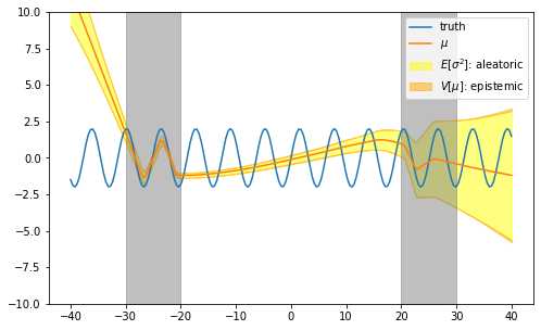
By using the Law of Total Variance we can decompose the aleatoric and epistemic components of the predicted uncertainty. With random-initialization we can see that epistemic uncertainty is almost null everywhere and not informative on area missing data (white background).
3.12. AutoDEUQ: Automated Deep Ensemble with Uncertainty Quantification#
AutoDEUQ is an algorithm in 2 steps: 1. joint hyperparameter and neural architecture search to generate a catalog of models. 2. build an ensemble from the catalog
To this end we start by editing slightly the previous RegressionFactory by adding the DistributionLambda layer as output.
[33]:
DistributionLambda = operation(tfp.layers.DistributionLambda)
[34]:
class RegressionUQSpace(KSearchSpace):

    def __init__(self, input_shape, output_shape, seed=None, num_layers=3):
        super().__init__(input_shape, output_shape, seed=seed)

        self.num_layers = 3

    def build(self):

        out_sub_graph = self.build_sub_graph(self.input_nodes[0], self.num_layers)

        output_dim = self.output_shape[0]
        output_dense = ConstantNode(op=Dense(output_dim*2))
        self.connect(out_sub_graph, output_dense)


        output_dist = ConstantNode(
            op=DistributionLambda(
                lambda t: tfd.Normal(
                    loc=t[..., :output_dim],
                    scale=1e-3 + tf.math.softplus(0.05 * t[..., output_dim:]),
                )
            )
        )
        self.connect(output_dense, output_dist)

        return self

    def build_sub_graph(self, input_node, num_layers=3):


        # Look over skip connections within a range of the 3 previous nodes
        anchor_points = collections.deque([input_node], maxlen=3)

        prev_node = input_node

        for _ in range(num_layers):

            # Create a variable node to list possible "Dense" layers
            dense = VariableNode()

            # Add the possible operations to the dense node
            self.add_dense_to_(dense)

            # Connect the previous node to the dense node
            self.connect(prev_node, dense)

            # Create a constant node to merge all input connections
            merge = ConstantNode()
            merge.set_op(
                AddByProjecting(self, [dense], activation="relu")
            )

            for node in anchor_points:

                # Create a variable node for each possible connection
                skipco = VariableNode()

                skipco.add_op(Zero()) # corresponds to no connection
                skipco.add_op(Connect(self, node)) # corresponds to (node => skipco)

                # Connect the (skipco => merge)
                self.connect(skipco, merge)


            # ! for next iter
            prev_node = merge
            anchor_points.append(prev_node)

        return prev_node

    def add_dense_to_(self, node):

        # We add the "Identity" operation to allow the choice "doing nothing"
        node.add_op(Identity())

        step = 16
        for units in range(step, step * 16 + 1, step):
            for activation in ACTIVATIONS:
                node.add_op(Dense(units=units, activation=activation))
For joint hyperparameter and neural architecture search it is possible to use the problem.add_hyperparameter(...) to define variable hyperparameters in the NAS Problem.
[35]:
problem_uq = NaProblem()

problem_uq.load_data(load_data_train_valid)

problem_uq.preprocessing(stdscaler)

problem_uq.search_space(RegressionUQSpace, num_layers=3)

problem_uq.hyperparameters(
    batch_size=problem_uq.add_hyperparameter((1, 32), "batch_size"),
    learning_rate=problem_uq.add_hyperparameter(
        (1e-4, 0.1, "log-uniform"),
        "learning_rate",
    ),
    optimizer=problem_uq.add_hyperparameter(
        ["sgd", "rmsprop", "adagrad", "adam", "adadelta", "adamax", "nadam"],
        "optimizer",
    ),
    patience_ReduceLROnPlateau=problem_uq.add_hyperparameter(
        (10, 20), "patience_ReduceLROnPlateau"
    ),
    patience_EarlyStopping=problem_uq.add_hyperparameter(
        (20, 30), "patience_EarlyStopping"
    ),
    epsilon=1e-7,
    num_epochs=200,
    callbacks=dict(
        ReduceLROnPlateau=dict(monitor="val_loss", mode="min", verbose=0, patience=5),
        EarlyStopping=dict(monitor="val_loss", mode="min", verbose=0, patience=10),
        # We save trained models in neural architecture search
        ModelCheckpoint=dict(
            monitor="val_loss",
            mode="min",
            save_best_only=True,
            verbose=0,
            filepath="model.h5",
            save_weights_only=False,
        ),
    ),
)

problem_uq.loss(nll)

problem_uq.metrics([])

# The objective is maximized so we take the negative of the validation loss
# where the loss is minimized
problem_uq.objective("-val_loss")

problem_uq
[35]:
Problem is:
    - search space   : __main__.RegressionUQSpace
    - data loading   : __main__.load_data_train_valid
    - preprocessing  : __main__.stdscaler
    - hyperparameters:
        * verbose: 0
        * batch_size: batch_size, Type: UniformInteger, Range: [1, 32], Default: 16
        * learning_rate: learning_rate, Type: UniformFloat, Range: [0.0001, 0.1], Default: 0.0031622777, on log-scale
        * optimizer: optimizer, Type: Categorical, Choices: {sgd, rmsprop, adagrad, adam, adadelta, adamax, nadam}, Default: sgd
        * patience_ReduceLROnPlateau: patience_ReduceLROnPlateau, Type: UniformInteger, Range: [10, 20], Default: 15
        * patience_EarlyStopping: patience_EarlyStopping, Type: UniformInteger, Range: [20, 30], Default: 25
        * num_epochs: 200
        * callbacks: {'ReduceLROnPlateau': {'monitor': 'val_loss', 'mode': 'min', 'verbose': 0, 'patience': 5}, 'EarlyStopping': {'monitor': 'val_loss', 'mode': 'min', 'verbose': 0, 'patience': 10}, 'ModelCheckpoint': {'monitor': 'val_loss', 'mode': 'min', 'save_best_only': True, 'verbose': 0, 'filepath': 'model.h5', 'save_weights_only': False}}
    - loss           : <function nll at 0x348e6f0d0>
    - metrics        :
    - objective      : -val_loss
[36]:
results_uq = {}
The max_evals has to be superior or equal to 400 to start having a good UQ estimate.
[37]:
from deephyper.search.nas import AgEBO


if os.path.exists("agebo_search"):
    shutil.rmtree("agebo_search")

# "n_jobs" is the number of processes used to refresh the state of the surrogate model used in AgEBO
agebo_search = AgEBO(problem_uq, get_evaluator(run_base_trainer), log_dir="agebo_search", n_jobs=4)

results_uq["agebo"] = agebo_search.search(max_evals=500)
/Users/romainegele/Documents/Argonne/deephyper/deephyper/evaluator/_evaluator.py:99: UserWarning: Applying nest-asyncio patch for IPython Shell!
  warnings.warn(
Created new evaluator with 4 workers and config: {'num_cpus': 1, 'num_cpus_per_task': 1, 'callbacks': [<deephyper.evaluator.callback.TqdmCallback object at 0x34491aa60>]}
[38]:
results_uq["agebo"]
[38]:
| arch_seq | batch_size | learning_rate | optimizer | patience_EarlyStopping | patience_ReduceLROnPlateau | job_id | objective | timestamp_submit | timestamp_gather | |
|---|---|---|---|---|---|---|---|---|---|---|
| 0 | [152, 1, 30, 0, 1, 113, 1, 1, 0] | 27 | 0.007159 | adagrad | 29 | 12 | 2 | -1.450841 | 0.173591 | 2.475589 |
| 1 | [66, 1, 135, 0, 1, 139, 0, 1, 0] | 25 | 0.000148 | nadam | 28 | 15 | 3 | -1.450301 | 0.173627 | 3.500935 |
| 2 | [56, 1, 37, 1, 1, 171, 0, 1, 1] | 18 | 0.002885 | rmsprop | 28 | 19 | 4 | -0.738564 | 0.173662 | 4.921706 |
| 3 | [43, 1, 116, 1, 0, 170, 1, 1, 0] | 13 | 0.000106 | rmsprop | 25 | 18 | 5 | -1.450331 | 2.657677 | 6.268550 |
| 4 | [118, 0, 17, 0, 0, 103, 0, 1, 0] | 32 | 0.000166 | adam | 22 | 13 | 7 | -1.455081 | 5.091059 | 6.817152 |
| ... | ... | ... | ... | ... | ... | ... | ... | ... | ... | ... |
| 495 | [26, 1, 162, 0, 0, 52, 1, 0, 1] | 5 | 0.003116 | rmsprop | 20 | 18 | 496 | -1.205748 | 932.602933 | 942.308652 |
| 496 | [60, 0, 162, 0, 0, 136, 1, 0, 0] | 6 | 0.003067 | rmsprop | 23 | 16 | 500 | -0.660088 | 943.115550 | 951.733516 |
| 497 | [60, 0, 162, 0, 1, 136, 1, 0, 1] | 5 | 0.003600 | rmsprop | 22 | 17 | 498 | -0.703299 | 938.832237 | 952.509710 |
| 498 | [26, 1, 162, 0, 0, 136, 1, 0, 0] | 1 | 0.002147 | rmsprop | 20 | 10 | 499 | -1.411145 | 939.592606 | 952.510410 |
| 499 | [60, 0, 162, 0, 0, 136, 1, 0, 0] | 2 | 0.002657 | rmsprop | 20 | 15 | 497 | -0.663001 | 933.405235 | 953.971765 |
500 rows × 10 columns
Different sizes of ensemble and two selection strategies can be experimented for ensembles: * caruana: a greedy selection from Caruana based on the loss function. * topk: select the top-k (i.e., size) best models based on the loss function.
[39]:
ensemble = UQBaggingEnsembleRegressor(
    model_dir="agebo_search/save/model",
    loss=nll,  # default is nll
    size=5,
    verbose=True,
    ray_address="auto",
    num_cpus=1,
    num_gpus=1 if is_gpu_available else None,
    selection="caruana",
)

ensemble.fit(s_vx, s_vy)

print(f"Selected {len(ensemble.members_files)} members are: ", ensemble.members_files)
Selected 5 members are: ['dc560236-e70f-11ec-a314-5e52ffa7b52c.h5', '2f251484-e710-11ec-a314-5e52ffa7b52c.h5', '2c4ed40c-e710-11ec-8e5f-5e52ffa7b52c.h5', 'fae39bdc-e70f-11ec-8e5f-5e52ffa7b52c.h5', 'd939d54c-e70e-11ec-a3ef-5e52ffa7b52c.h5']
[40]:
pred_s_ty, pred_s_ty_aleatoric_var, pred_s_ty_epistemic_var = ensemble.predict_var_decomposition(s_tx)

pred_ty_mean = pred_s_ty.loc.numpy() + scaler_y.mean_
pred_ty_aleatoric_var = pred_s_ty_aleatoric_var * scaler_y.var_
pred_ty_epistemic_var = pred_s_ty_epistemic_var * scaler_y.var_

width = 8
height = width/1.618
plt.figure(figsize=(width, height))

plt.plot(tx, ty, label="truth")
plt.plot(tx, pred_ty_mean, label="$\mu$")
plt.fill_between(
    tx.reshape(-1),
    (pred_ty_mean - pred_ty_aleatoric_var).reshape(-1),
    (pred_ty_mean + pred_ty_aleatoric_var).reshape(-1),
    color="yellow",
    alpha=0.5,
    label="$E[\sigma^2]$: aleatoric"
)
plt.fill_between(
    tx.reshape(-1),
    (pred_ty_mean - pred_ty_aleatoric_var).reshape(-1),
    (pred_ty_mean - pred_ty_aleatoric_var - pred_ty_epistemic_var).reshape(-1),
    color="orange",
    alpha=0.5,
    label="$V[\mu]$: epistemic"
)
plt.fill_between(
    tx.reshape(-1),
    (pred_ty_mean + pred_ty_aleatoric_var).reshape(-1),
    (pred_ty_mean + pred_ty_aleatoric_var + pred_ty_epistemic_var).reshape(-1),
    color="orange",
    alpha=0.5,
)

y_lim = 10
plt.fill_between([-30, -20], [-y_lim, -y_lim], [y_lim, y_lim], color="grey", alpha=0.5)
plt.fill_between([20, 30], [-y_lim, -y_lim], [y_lim, y_lim], color="grey", alpha=0.5)

plt.legend()
plt.ylim(-y_lim, y_lim)

plt.show()
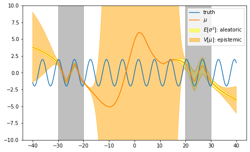
We notice that adding more diversity in the catalog can help have much better epistemic uncertainty estimates.
3.13. Random Forest#
What if we compare this to using the same technic (i.e., law of total variance) on the trees used to build a random forest regressor.
[45]:
import warnings

from deephyper.skopt.learning import RandomForestRegressor

with warnings.catch_warnings():
    warnings.simplefilter("ignore")

    rf_model = RandomForestRegressor()

    rf_model.fit(s_x, s_y)
[46]:
pred_s_ty, pred_s_ty_std = rf_model.predict(s_tx, return_std=True)
pred_s_ty_var = pred_s_ty_std ** 2
[47]:
pred_ty_mean = pred_s_ty + scaler_y.mean_
pred_ty_var = pred_s_ty_var * scaler_y.var_

width = 8
height = width/1.618
plt.figure(figsize=(width, height))

plt.plot(tx, ty, label="truth")
plt.plot(tx, pred_ty_mean, label="$\mu$")
plt.fill_between(
    tx.reshape(-1),
    (pred_ty_mean - pred_ty_var).reshape(-1),
    (pred_ty_mean + pred_ty_var).reshape(-1),
    color="yellow",
    alpha=0.5,
    label="$\sigma^2$"
)

y_lim = 10
plt.fill_between([-30, -20], [-y_lim, -y_lim], [y_lim, y_lim], color="grey", alpha=0.5)
plt.fill_between([20, 30], [-y_lim, -y_lim], [y_lim, y_lim], color="grey", alpha=0.5)

plt.legend()
plt.ylim(-y_lim, y_lim)

plt.show()
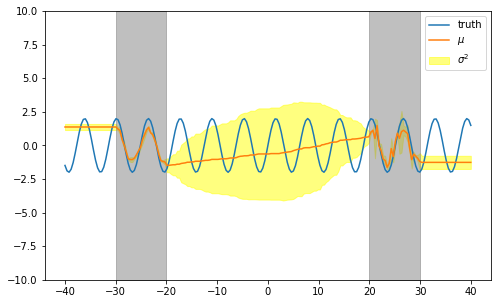
We can see that the uncertainty estimate is really poor in this case.