
Neural Architecture Search for Graph Neural Networks#
In this tutorial, we will design neural architecture search spaces for graph neural networks, specifically for message passing neural networks.
For related papers, please check https://ieeexplore.ieee.org/abstract/document/9378060.
The search space have multiple input tensors, including node features, edge features, edge pairs (source and target node indices) and node masks (number of nodes before zero-padding). The output of this search space is customizable. In this tutorial, we use an example from the QM7 dataset, which has a scalar output. The QM7 dataset is from the Deepchem library.
There are two main variable nodes, namely mpnn_cell and gather_cell: * mpnn_cell is a message passing layer with a varierty of activation, aggregation, update functions, etc. * gather_cell is global graph gather layer with a variety of global pooling functions.
We also adopted skip-connection in the search space; that is, the output of the n-1 layer is the direct input to the n+1 layer. Users can modify the number of mpnn_cell and maximum skip-connection distance to control the flexibility of skip-connection.
We used random search and aging evolution (regularized evolution) to conduct architecture search. In the paper, we found aging evolution has good scalability. We also showed that the best architecture from the search outperforms the moleculenet benchmarks. Users are more than welcome to furthur modify the search space to boost the performance.
Install Deepchem and RDKit#
We need DeepChem for the benchmark datasets. RDKit is also required to convert molecule smile string to a graph representation.
[1]:
!pip install deepchem
!conda install -c rdkit rdkit -y
Requirement already satisfied: deepchem in /Users/romainegele/miniforge3/envs/dh-arm/lib/python3.9/site-packages (2.5.0)
Requirement already satisfied: joblib in /Users/romainegele/miniforge3/envs/dh-arm/lib/python3.9/site-packages (from deepchem) (1.1.0)
Requirement already satisfied: scipy in /Users/romainegele/miniforge3/envs/dh-arm/lib/python3.9/site-packages (from deepchem) (1.7.2)
Requirement already satisfied: pandas in /Users/romainegele/miniforge3/envs/dh-arm/lib/python3.9/site-packages (from deepchem) (1.3.4)
Requirement already satisfied: numpy in /Users/romainegele/miniforge3/envs/dh-arm/lib/python3.9/site-packages (from deepchem) (1.21.4)
Requirement already satisfied: scikit-learn in /Users/romainegele/miniforge3/envs/dh-arm/lib/python3.9/site-packages (from deepchem) (1.0.1)
Requirement already satisfied: python-dateutil>=2.7.3 in /Users/romainegele/miniforge3/envs/dh-arm/lib/python3.9/site-packages (from pandas->deepchem) (2.8.2)
Requirement already satisfied: pytz>=2017.3 in /Users/romainegele/miniforge3/envs/dh-arm/lib/python3.9/site-packages (from pandas->deepchem) (2021.3)
Requirement already satisfied: threadpoolctl>=2.0.0 in /Users/romainegele/miniforge3/envs/dh-arm/lib/python3.9/site-packages (from scikit-learn->deepchem) (3.0.0)
Requirement already satisfied: six>=1.5 in /Users/romainegele/miniforge3/envs/dh-arm/lib/python3.9/site-packages (from python-dateutil>=2.7.3->pandas->deepchem) (1.15.0)
Collecting package metadata (current_repodata.json): done
Solving environment: done


==> WARNING: A newer version of conda exists. <==
  current version: 4.10.3
  latest version: 4.11.0

Please update conda by running

    $ conda update -n base conda


# All requested packages already installed.
Imports and GPU Detection#
Warning
By design asyncio does not allow nested event loops. Jupyter is using Tornado which already starts an event loop. Therefore the following patch is required to run this tutorial.
[2]:
!pip install nest_asyncio

import nest_asyncio
nest_asyncio.apply()
Requirement already satisfied: nest_asyncio in /Users/romainegele/miniforge3/envs/dh-arm/lib/python3.9/site-packages (1.5.1)
[3]:
import json
import os
import pathlib
import shutil

!export TF_CPP_MIN_LOG_LEVEL=3
!export TF_XLA_FLAGS=--tf_xla_enable_xla_devices

import matplotlib.pyplot as plt
import numpy as np
import tensorflow as tf
from tqdm import tqdm
Note
The TF_CPP_MIN_LOG_LEVEL can be used to avoid the logging of Tensorflow DEBUG, INFO and WARNING statements.
Note
The following can be used to detect if GPU devices are available on the current host.
[4]:
import tensorflow as tf

available_gpus = tf.config.list_physical_devices("GPU")
n_gpus = len(available_gpus)

if n_gpus > 1:
    n_gpus -= 1
is_gpu_available = n_gpus > 0

if is_gpu_available:
    print(f"{n_gpus} GPU{'s are' if n_gpus > 1 else ' is'} available.")
else:
    print("No GPU available")
No GPU available
Start Ray#
We launch the Ray run-time depending on the detected local ressources. If GPU(s) is(are) detected then 1 worker is started for each GPU. If not, then only 1 worker is started. You can start more workers by setting num_cpus=1 to a value greater than 1.
Warning
In the case of GPUs it is important to follow this scheme to avoid multiple processes (Ray workers vs current process) to lock the same GPU.
[5]:
import ray

log_to_driver = False

if not(ray.is_initialized()):
    if is_gpu_available:
        ray.init(num_cpus=n_gpus, num_gpus=n_gpus, log_to_driver=log_to_driver)
    else:
        ray.init(num_cpus=1, log_to_driver=log_to_driver)
2021-12-13 11:47:14,280 INFO services.py:1338 -- View the Ray dashboard at http://127.0.0.1:8265
Reformatting Graph Dataset#
Now, we will start by reformatting a benchmark QM7 from molecule-net. We will first generate data for a training set (used for estimation) and a testing set (used to evaluate the final performance). Then the training set will be sub-divided in a new training set (used to estimate the neural network weights) and validation set (used to estimate the neural network hyperparameters and architecture).
The data is converted from a deepchem weave object to a list containing node features, edge features, edge pairs, node masks and GCN attention coefficients. You may check the details here https://ieeexplore.ieee.org/abstract/document/9378060
[6]:
from deepchem.molnet import load_qm7
from deephyper.contrib.mpnn import get_all_mol_feat


def load_data(test_only=0, verbose=0):
    _, (train_data, valid_data, test_data), _ = load_qm7(featurizer='Weave',
                                                         splitter='random')

    max_node, max_edge = [], [] # used to zero-pad the node and edge features to maximum dimension

    for data in [train_data, valid_data, test_data]:
        x = data.X
        size = len(x) # number of molecules in a dataset
        max_node.append(np.max([x[i].nodes.shape[0] for i in range(size)]))
        max_edge.append(np.max([x[i].pairs.shape[0] for i in range(size)]))
    max_node = np.max(max_node)
    max_edge = np.max(max_edge)

    x_train, y_train = get_all_mol_feat(train_data, max_node, max_edge)
    x_valid, y_valid = get_all_mol_feat(valid_data, max_node, max_edge)
    x_test, y_test = get_all_mol_feat(test_data, max_node, max_edge)

    if verbose:
        print(f'x_train shape: {[x.shape for x in x_train]}')
        print(f'y_train shape: {y_train.shape}')
        print(f'x_valid shape: {[x.shape for x in x_valid]}')
        print(f'y_valid shape: {y_valid.shape}')
        print(f'x_test shape: {[x.shape for x in x_test]}')
        print(f'y_test shape: {y_test.shape}')

    if test_only:
        return (x_test, y_test)
    else:
        return (x_train, y_train), (x_valid, y_valid)
Then the code to split the training data in a new training set and a validation set corresponds to:
[7]:
# ignore warning/errors when downloading the dataset for the first time
(x, y), (vx, vy) = load_data(verbose=1)
(tx , ty) = load_data(test_only=1)
x_train shape: [(5470, 22, 75), (5470, 506, 2), (5470, 506, 14), (5470, 22), (5470, 506)]
y_train shape: (5470, 1)
x_valid shape: [(684, 22, 75), (684, 506, 2), (684, 506, 14), (684, 22), (684, 506)]
y_valid shape: (684, 1)
x_test shape: [(684, 22, 75), (684, 506, 2), (684, 506, 14), (684, 22), (684, 506)]
y_test shape: (684, 1)
Note
When it is possible to factorize the two previous function into one, DeepHyper interface requires a function which returns (train_inputs, train_outputs), (valid_inputs, valid_outputs).
Baseline Neural Network#
Let us define a baseline neural network based on a regular multi-layer perceptron architecture which learn the mean estimate and minimise the mean squared error.
[8]:
import deephyper.layers as dhl
from tensorflow.keras.callbacks import ModelCheckpoint
[9]:
def gnn_default_model(shape):
    node_ = tf.keras.layers.Input(shape[0])
    adj_ = tf.keras.layers.Input(shape[1], dtype=tf.int32)
    edge_ = tf.keras.layers.Input(shape[2])
    mask_ = tf.keras.layers.Input(shape[3])
    degree_ = tf.keras.layers.Input(shape[4])

    input_ = [node_, adj_, edge_, mask_, degree_]

    node = dhl.SparseMPNN(state_dim=32,
                       T=1,
                       aggr_method='max',
                       attn_method='const',
                       update_method='gru',
                       attn_head=1,
                       activation='elu')([node_, adj_, edge_, mask_, degree_])

    node = dhl.GlobalAttentionPool(128)(node)
    node = tf.keras.layers.Flatten()(node)
    node = tf.keras.layers.Dense(32, activation='relu')(node)

    output = tf.keras.layers.Dense(1, activation='linear')(node)

    model = tf.keras.Model(input_, output)

    return model


shape = [item.shape[1:] for item in x]
model = gnn_default_model(shape)

model.compile(optimizer="adam", loss='mse')
mc = ModelCheckpoint('gnn_model.h5', monitor='val_loss', mode='min', save_weights_only=True)

history = model.fit(x, y,
                    epochs=5,
                    batch_size=128,
                    validation_data=(vx, vy),
                    verbose=1,
                    callbacks=[mc]).history
2021-12-13 11:47:19.988355: I tensorflow/compiler/mlir/mlir_graph_optimization_pass.cc:185] None of the MLIR Optimization Passes are enabled (registered 2)
2021-12-13 11:47:19.988498: W tensorflow/core/platform/profile_utils/cpu_utils.cc:128] Failed to get CPU frequency: 0 Hz
Epoch 1/5
43/43 [==============================] - 5s 106ms/step - loss: 1.0011 - val_loss: 1.0239
Epoch 2/5
43/43 [==============================] - 4s 102ms/step - loss: 0.9441 - val_loss: 0.9451
Epoch 3/5
43/43 [==============================] - 4s 105ms/step - loss: 0.9161 - val_loss: 0.9458
Epoch 4/5
43/43 [==============================] - 5s 105ms/step - loss: 0.8961 - val_loss: 0.9464
Epoch 5/5
43/43 [==============================] - 5s 108ms/step - loss: 0.9018 - val_loss: 0.9554
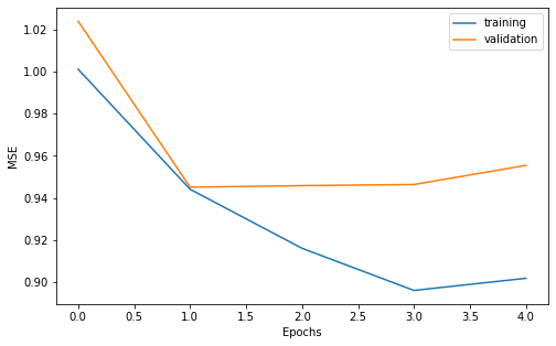
We can do a vizualisation of our learning curves to make sure the training and validation loss decrease correctly.
[10]:
width = 8
height = width/1.618
plt.figure(figsize=(width, height))

plt.plot(history["loss"], label="training")
plt.plot(history["val_loss"], label="validation")

plt.xlabel("Epochs")
plt.ylabel("MSE")

plt.legend()

plt.show()
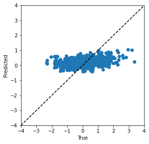
Also, let us look at the prediction on the test set.
[11]:
model.load_weights('gnn_model.h5')
pred_ty = model.predict(tx)

width = 4.5
height = width
plt.figure(figsize=(width, height))

vmin, vmax = -4, 4
plt.scatter(ty, pred_ty)
plt.plot([vmin, vmax], [vmin, vmax], 'k--')
plt.xlim([vmin, vmax])
plt.ylim([vmin, vmax])
plt.xlabel('True')
plt.ylabel('Predicted')

plt.show()
Define the Neural Architecture Search Space#
The neural architecture search space is composed of discrete decision variables. For each decision variable we choose among a list of possible operation to perform (e.g., fully connected, ReLU). To define this search space, it is necessary to use two classes:
KSearchSpace(for Keras Search Space): represents a directed acyclic graph (DAG) in which each node represents a chosen operation. It represents the possible neural networks that can be created.SpaceFactory: is a utilitiy class used to pack the logic of a search space definition and share it with others.
Then, inside a KSearchSpace we will have two types of nodes: * VariableNode: corresponds to discrete decision variables and are used to define a list of possible operation. * ConstantNode: corresponds to fixed operation in the search space (e.g., input/outputs)
Finally, it is possible to reuse any tf.keras.layers to define a KSearchSpace. However, it is important to wrap each layer in an operation to perform a lazy memory allocation of tensors.
We implement the constructor __init__ and build method of the RegressionSpace a subclass of KSearchSpace. The __init__ method interface is:
def __init__(self, input_shape, output_shape, **kwargs):
    ...
for the build method the interface is:
def build(self):
    ...
    return self
where: * input_shape corresponds to a tuple or a list of tuple indicating the shapes of inputs tensors. * output_shape corresponds to the same but of output_tensors. * **kwargs denotes that any other key word argument can be defined by the user.
[12]:
import collections, itertools

from deephyper.nas import KSearchSpace
from deephyper.nas.node import ConstantNode, VariableNode
from deephyper.nas.operation import operation, Zero, Connect, AddByProjecting, Identity

# define operations
Flatten = operation(tf.keras.layers.Flatten)
Dense = operation(tf.keras.layers.Dense)

SparseMPNN = operation(dhl.SparseMPNN)
GlobalAttentionPool = operation(dhl.GlobalAttentionPool)
GlobalAttentionSumPool = operation(dhl.GlobalAttentionSumPool)
GlobalAvgPool = operation(dhl.GlobalAvgPool)
GlobalMaxPool = operation(dhl.GlobalMaxPool)
GlobalSumPool = operation(dhl.GlobalSumPool)

class MPNNSpace(KSearchSpace):

    def __init__(self, input_shape, output_shape, seed=None, num_layers=3):
        super().__init__(input_shape, output_shape, seed=seed)
        self.num_layers = 3

    def build(self):

        source = prev_input = self.input_nodes[0]
        prev_input1 = self.input_nodes[1]
        prev_input2 = self.input_nodes[2]
        prev_input3 = self.input_nodes[3]
        prev_input4 = self.input_nodes[4]

        anchor_points = collections.deque([source], maxlen=3)

        for _ in range(self.num_layers):
            graph_attn_cell = VariableNode()
            self.mpnn_cell(graph_attn_cell)
            self.connect(prev_input, graph_attn_cell)
            self.connect(prev_input1, graph_attn_cell)
            self.connect(prev_input2, graph_attn_cell)
            self.connect(prev_input3, graph_attn_cell)
            self.connect(prev_input4, graph_attn_cell)

            merge = ConstantNode()
            merge.set_op(AddByProjecting(self, [graph_attn_cell], activation="relu"))

            for node in anchor_points:
                skipco = VariableNode()
                skipco.add_op(Zero())
                skipco.add_op(Connect(self, node))
                self.connect(skipco, merge)

            prev_input = merge

            anchor_points.append(prev_input)

        global_pooling_node = VariableNode()
        self.gather_cell(global_pooling_node)
        self.connect(prev_input, global_pooling_node)
        prev_input = global_pooling_node

        flatten_node = ConstantNode(Flatten())
        self.connect(prev_input, flatten_node)

        # Output
        output = ConstantNode(Dense(self.output_shape[0]))
        self.connect(flatten_node, output)

        return self

    def mpnn_cell(self, node):
        state_dims = [4, 8, 16, 32]
        Ts = [1, 2, 3, 4]
        attn_methods = ["const", "gat", "sym-gat", "linear", "gen-linear", "cos"]
        attn_heads = [1, 2, 4, 6]
        aggr_methods = ["max", "mean", "sum"]
        update_methods = ["gru", "mlp"]
        activations = [tf.keras.activations.sigmoid,
                       tf.keras.activations.tanh,
                       tf.keras.activations.relu,
                       tf.keras.activations.linear,
                       tf.keras.activations.elu,
                       tf.keras.activations.softplus,
                       tf.nn.leaky_relu,
                       tf.nn.relu6]

        for hp in itertools.product(state_dims,
                                    Ts,
                                    attn_methods,
                                    attn_heads,
                                    aggr_methods,
                                    update_methods,
                                    activations):
            (state_dim, T, attn_method, attn_head, aggr_method, update_method, activation) = hp

            node.add_op(
                SparseMPNN(
                    state_dim=state_dim,
                    T=T,
                    attn_method=attn_method,
                    attn_head=attn_head,
                    aggr_method=aggr_method,
                    update_method=update_method,
                    activation=activation
                )
            )


    def gather_cell(self, node):
        for functions in [GlobalSumPool, GlobalMaxPool, GlobalAvgPool]:
            for axis in [-1, -2]:
                node.add_op(functions(axis=axis))
        node.add_op(Flatten())

        for state_dim in [16, 32, 64]:
            node.add_op(GlobalAttentionPool(state_dim=state_dim))
        node.add_op(GlobalAttentionSumPool())
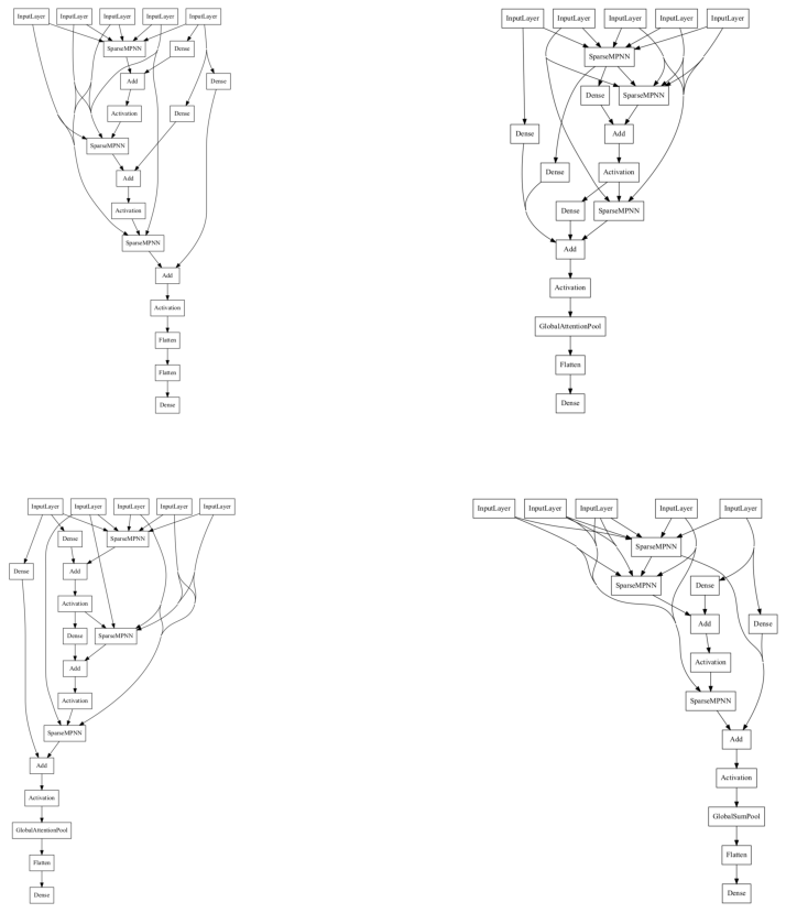
Let us visualize a few randomly sampled neural architecture from this search space.
[13]:
import matplotlib.image as mpimg
from tensorflow.keras.utils import plot_model

input_shape = [item.shape[1:] for item in x]
output_shape = y.shape[1:]
shapes = dict(input_shape=input_shape, output_shape=output_shape)
space = MPNNSpace(**shapes).build()

print(space.choices())


images = []
plt.figure(figsize=(15,15))
for i in range(4):

    model = space.sample()
    plt.subplot(2,2,i+1)
    plot_model(model, "random_model.png", show_shapes=False, show_layer_names=False)
    image = mpimg.imread("random_model.png")
    plt.imshow(image)
    plt.axis('off')

plt.show()
[(0, 18431), (0, 1), (0, 18431), (0, 1), (0, 1), (0, 18431), (0, 1), (0, 1), (0, 1), (0, 10)]
Define the Neural Architecture Optimization Problem#
In order to define a neural architecture search problem we have to use the NaProblem class. This class gives access to different method for the user to customize the training settings of neural networks.
[14]:
from deephyper.problem import NaProblem

problem = NaProblem()

# Bind a function which returns (train_input, train_output), (valid_input, valid_output)
problem.load_data(load_data)

# Bind a function which returns a search space and give some arguments for the `build` method
problem.search_space(MPNNSpace, num_layers=2)

# Define a set of fixed hyperparameters for all trained neural networks
problem.hyperparameters(
    batch_size=128,
    learning_rate=1e-3,
    optimizer="adam",
    num_epochs=1, # lower fidelity
)

# Define the loss to minimize
problem.loss("mse")

# Define complementary metrics
problem.metrics([])

# Define the maximized objective. Here we take the negative of the validation loss.
problem.objective("-val_loss")

problem
[14]:
Problem is:
    - search space   : __main__.MPNNSpace
    - data loading   : __main__.load_data
    - preprocessing  : None
    - hyperparameters:
        * verbose: 0
        * batch_size: 128
        * learning_rate: 0.001
        * optimizer: adam
        * num_epochs: 1
    - loss           : mse
    - metrics        :
    - objective      : -val_loss
Tip
Adding an EarlyStopping(...) callback is a good idea to stop the training of your model as soon as it stops to improve.
...
EarlyStopping=dict(monitor="val_loss", mode="min", verbose=0, patience=3)
...
Define the Evaluator Object#
The Evaluator object is responsible of defining the backend used to distribute the function evaluation in DeepHyper.
[15]:
from deephyper.evaluator import Evaluator
from deephyper.evaluator.callback import LoggerCallback


def get_evaluator(run_function):

    # Default arguments for Ray: 1 worker and 1 worker per evaluation
    method_kwargs = {
        "num_cpus": 1,
        "num_cpus_per_task": 1,
        "callbacks": [LoggerCallback()] # To interactively follow the finished evaluations,
    }

    # If GPU devices are detected then it will create 'n_gpus' workers
    # and use 1 worker for each evaluation
    if is_gpu_available:
        method_kwargs["num_cpus"] = n_gpus
        method_kwargs["num_gpus"] = n_gpus
        method_kwargs["num_cpus_per_task"] = 1
        method_kwargs["num_gpus_per_task"] = 1

    evaluator = Evaluator.create(
        run_function,
        method="ray",
        method_kwargs=method_kwargs
    )
    print(f"Created new evaluator with {evaluator.num_workers} worker{'s' if evaluator.num_workers > 1 else ''} and config: {method_kwargs}", )

    return evaluator
For neural architecture search a standard training pipeline is provided by the run_base_trainer function from the deephyper.nas.run module.
[16]:
from deephyper.nas.run import run_base_trainer
Define and Run the Neural Architecture Search#
All search algorithms follow a similar interface. A problem and evaluator object has to be provided to the search then the search can be executed through the search(max_evals, timeout) method.
[17]:
results = {} # used to store the results of different search algorithms
max_evals = 10 # maximum number of iteratins for all searches
[18]:
from deephyper.search.nas import Random

random_search = Random(problem, get_evaluator(run_base_trainer), log_dir="random_search")

results["random"] = random_search.search(max_evals=max_evals)
Created new evaluator with 1 worker and config: {'num_cpus': 1, 'num_cpus_per_task': 1, 'callbacks': [<deephyper.evaluator.callback.LoggerCallback object at 0x293060100>]}
[00001] -- best objective: -1.01752 -- received objective: -1.01752
[00002] -- best objective: -1.01752 -- received objective: -1.04781
[00003] -- best objective: -1.00011 -- received objective: -1.00011
[00004] -- best objective: -0.92881 -- received objective: -0.92881
[00005] -- best objective: -0.92881 -- received objective: -1.04169
[00006] -- best objective: -0.92881 -- received objective: -1.07058
[00007] -- best objective: -0.92881 -- received objective: -1.27250
[00008] -- best objective: -0.92881 -- received objective: -1.07548
[00009] -- best objective: -0.92881 -- received objective: -0.99138
[00010] -- best objective: -0.92881 -- received objective: -0.99931
If we look at the dataframe of results for each search we will find it slightly different than the one of hyperparameter search. A new column arch_seq corresponds to an embedding for each evaluated architecture. Each integer of an arch_seq list corresponds to the choice of a VariableNode in our KSearchSpace.
[19]:
results["random"]
[19]:
| arch_seq | id | objective | elapsed_sec | duration | |
|---|---|---|---|---|---|
| 0 | [13876, 0, 2160, 0, 0, 4762, 0, 1, 1, 1] | 1 | -1.017522 | 44.933679 | 43.074681 |
| 1 | [5937, 0, 16471, 1, 0, 9397, 1, 1, 0, 2] | 2 | -1.047807 | 281.613137 | 236.678758 |
| 2 | [6123, 1, 1777, 1, 0, 9158, 0, 1, 1, 7] | 3 | -1.000114 | 339.803210 | 58.188634 |
| 3 | [5796, 1, 18368, 1, 1, 15679, 0, 1, 1, 6] | 4 | -0.928806 | 579.374068 | 239.570209 |
| 4 | [7159, 1, 1494, 0, 0, 9234, 0, 1, 1, 4] | 5 | -1.041694 | 611.826204 | 32.451197 |
| 5 | [4662, 0, 7258, 0, 0, 2419, 1, 1, 1, 5] | 6 | -1.070579 | 658.328865 | 46.501993 |
| 6 | [5898, 0, 12026, 1, 0, 4872, 1, 0, 1, 7] | 7 | -1.272499 | 710.819948 | 52.490447 |
| 7 | [6942, 1, 1192, 0, 0, 5577, 0, 1, 1, 5] | 8 | -1.075484 | 725.114781 | 14.294140 |
| 8 | [10451, 1, 12804, 1, 0, 5329, 1, 0, 1, 10] | 9 | -0.991375 | 796.194318 | 71.078856 |
| 9 | [6617, 1, 2963, 0, 0, 6786, 1, 1, 0, 3] | 10 | -0.999313 | 824.445577 | 28.250628 |
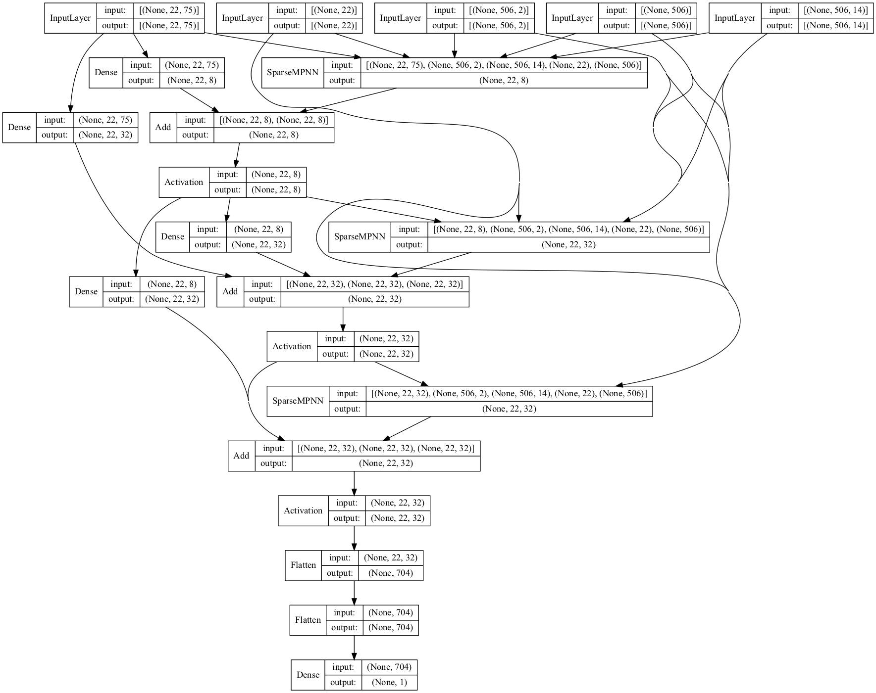
Let us visualize the best architecture found:
[20]:
i_max = results["random"].objective.argmax()
best_score = results["random"].iloc[i_max].objective
best_arch_seq = json.loads(results["random"].iloc[i_max].arch_seq)

best_model = space.sample(best_arch_seq)
plot_model(best_model, show_shapes=True, show_layer_names=False)
[20]:
[ ]:
best_model.compile(optimizer="adam", loss='mse')
mc = ModelCheckpoint('gnn_best_model.h5', monitor='val_loss', mode='min', save_weights_only=True)

history_best = best_model.fit(x, y,
                    epochs=50,
                    batch_size=128,
                    validation_data=(vx, vy),
                    verbose=1,
                    callbacks=[mc]).history
Epoch 1/50
43/43 [==============================] - 91s 2s/step - loss: 0.9519 - val_loss: 0.9487
Epoch 2/50
43/43 [==============================] - 93s 2s/step - loss: 0.8702 - val_loss: 0.8870
Epoch 3/50
43/43 [==============================] - 85s 2s/step - loss: 0.8189 - val_loss: 0.8192
Epoch 4/50
43/43 [==============================] - 84s 2s/step - loss: 0.7917 - val_loss: 0.7964
Epoch 5/50
43/43 [==============================] - 82s 2s/step - loss: 0.7909 - val_loss: 0.7834
Epoch 6/50
43/43 [==============================] - 84s 2s/step - loss: 0.7709 - val_loss: 0.7724
Epoch 7/50
43/43 [==============================] - 84s 2s/step - loss: 0.7605 - val_loss: 0.7746
Epoch 8/50
43/43 [==============================] - 83s 2s/step - loss: 0.7524 - val_loss: 0.7662
Epoch 9/50
43/43 [==============================] - 84s 2s/step - loss: 0.7487 - val_loss: 0.7601
Epoch 10/50
43/43 [==============================] - 84s 2s/step - loss: 0.7488 - val_loss: 0.7609
Epoch 11/50
43/43 [==============================] - 83s 2s/step - loss: 0.7414 - val_loss: 0.7677
Epoch 12/50
43/43 [==============================] - 82s 2s/step - loss: 0.7424 - val_loss: 0.7504
Epoch 13/50
43/43 [==============================] - 81s 2s/step - loss: 0.7314 - val_loss: 0.7356
Epoch 14/50
43/43 [==============================] - 81s 2s/step - loss: 0.7280 - val_loss: 0.7458
Epoch 15/50
43/43 [==============================] - 81s 2s/step - loss: 0.7263 - val_loss: 0.7381
Epoch 16/50
43/43 [==============================] - 83s 2s/step - loss: 0.7241 - val_loss: 0.7443
Epoch 17/50
43/43 [==============================] - 83s 2s/step - loss: 0.7212 - val_loss: 0.7343
Epoch 18/50
43/43 [==============================] - 83s 2s/step - loss: 0.7138 - val_loss: 0.7494
Epoch 19/50
43/43 [==============================] - 87s 2s/step - loss: 0.7073 - val_loss: 0.7442
Epoch 20/50
43/43 [==============================] - 84s 2s/step - loss: 0.7147 - val_loss: 0.7518
Epoch 21/50
43/43 [==============================] - 101s 2s/step - loss: 0.7149 - val_loss: 0.7477
Epoch 22/50
43/43 [==============================] - 108s 3s/step - loss: 0.7036 - val_loss: 0.7551
Epoch 23/50
43/43 [==============================] - 96s 2s/step - loss: 0.6998 - val_loss: 0.7245
Epoch 24/50
43/43 [==============================] - 89s 2s/step - loss: 0.6934 - val_loss: 0.7366
Epoch 25/50
43/43 [==============================] - 110s 3s/step - loss: 0.6904 - val_loss: 0.7511
Epoch 26/50
43/43 [==============================] - 90s 2s/step - loss: 0.6902 - val_loss: 0.7313
Epoch 27/50
43/43 [==============================] - 121s 3s/step - loss: 0.6898 - val_loss: 0.7531
Epoch 28/50
43/43 [==============================] - 103s 2s/step - loss: 0.6891 - val_loss: 0.7624
Epoch 29/50
43/43 [==============================] - 96s 2s/step - loss: 0.6809 - val_loss: 0.7437
Epoch 30/50
43/43 [==============================] - 169s 4s/step - loss: 0.6823 - val_loss: 0.7417
Epoch 31/50
43/43 [==============================] - 90s 2s/step - loss: 0.6784 - val_loss: 0.7530
Epoch 32/50
43/43 [==============================] - 142s 2s/step - loss: 0.6726 - val_loss: 0.7621
Epoch 33/50
43/43 [==============================] - 130s 3s/step - loss: 0.6721 - val_loss: 0.7374
Epoch 34/50
43/43 [==============================] - 95s 2s/step - loss: 0.6696 - val_loss: 0.7525
Epoch 35/50
43/43 [==============================] - 125s 3s/step - loss: 0.6667 - val_loss: 0.7607
Epoch 36/50
43/43 [==============================] - 90s 2s/step - loss: 0.6716 - val_loss: 0.7414
Epoch 37/50
43/43 [==============================] - 132s 2s/step - loss: 0.6580 - val_loss: 0.7319
Epoch 38/50
43/43 [==============================] - 129s 3s/step - loss: 0.6563 - val_loss: 0.7527
Epoch 39/50
43/43 [==============================] - 97s 2s/step - loss: 0.6595 - val_loss: 0.7719
Epoch 40/50
43/43 [==============================] - 97s 2s/step - loss: 0.6614 - val_loss: 0.7665
Epoch 41/50
43/43 [==============================] - 83s 2s/step - loss: 0.6496 - val_loss: 0.7620
Epoch 42/50
20/43 [============>.................] - ETA: 42s - loss: 0.6322
[ ]:
width = 8
height = width/1.618
plt.figure(figsize=(width, height))

plt.plot(history["val_loss"], label="Default Model")
plt.plot(history_best["val_loss"], label="Best Model")

plt.xlabel("Epochs")
plt.ylabel("MSE")

plt.legend()

plt.show()
[ ]:
best_model.load_weights('gnn_best_model.h5')
pred_ty = best_model.predict(tx)

width = 4.5
height = width
plt.figure(figsize=(width, height))

vmin, vmax = -4, 4
plt.scatter(ty, pred_ty)
plt.plot([vmin, vmax], [vmin, vmax], 'k--')
plt.xlim([vmin, vmax])
plt.ylim([vmin, vmax])
plt.xlabel('True')
plt.ylabel('Predicted')

plt.show()