
Note
Go to the end to download the full example code
Profile the Worker Utilization#
Author(s): Romain Egele.
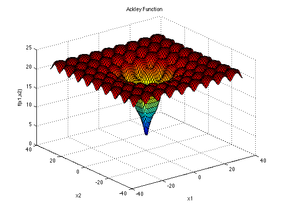
This example demonstrates the advantages of parallel evaluations over serial evaluations. We start by defining an artificial black-box run-function by using the Ackley function:
We will use the time.sleep function to simulate a budget of 2 secondes of execution in average which helps illustrate the advantage of parallel evaluations. The @profile decorator is useful to collect starting/ending time of the run-function execution which help us know exactly when we are inside the black-box. This decorator is necessary when profiling the worker utilization. When using this decorator, the run-function will return a dictionnary with 2 new keys "timestamp_start" and "timestamp_end". The run-function is defined in a separate module because of the “multiprocessing” backend that we are using in this example.
 1"""Set of Black-Box functions useful to build examples.
 2"""
 3import time
 4import numpy as np
 5from deephyper.evaluator import profile
 6
 7
 8def ackley(x, a=20, b=0.2, c=2 * np.pi):
 9    d = len(x)
10    s1 = np.sum(x**2)
11    s2 = np.sum(np.cos(c * x))
12    term1 = -a * np.exp(-b * np.sqrt(s1 / d))
13    term2 = -np.exp(s2 / d)
14    y = term1 + term2 + a + np.exp(1)
15    return y
16
17
18@profile
19def run_ackley(config, sleep_loc=2, sleep_scale=0.5):
20
21    # to simulate the computation of an expensive black-box
22    if sleep_loc > 0:
23        t_sleep = np.random.normal(loc=sleep_loc, scale=sleep_scale)
24        t_sleep = max(t_sleep, 0)
25        time.sleep(t_sleep)
26
27    x = np.array([config[k] for k in config if "x" in k])
28    x = np.asarray_chkfinite(x)  # ValueError if any NaN or Inf
29    return -ackley(x)  # maximisation is performed
After defining the black-box we can continue with the definition of our main script:
import black_box_util as black_box

from deephyper.analysis._matplotlib import update_matplotlib_rc

update_matplotlib_rc()
Then we define the variable(s) we want to optimize. For this problem we optimize Ackley in a 2-dimensional search space, the true minimul is located at (0, 0).
Configuration space object:
  Hyperparameters:
    x0, Type: UniformFloat, Range: [-32.768, 32.768], Default: 0.0
    x1, Type: UniformFloat, Range: [-32.768, 32.768], Default: 0.0
Then we define a parallel search.
if __name__ == "__main__":
    from deephyper.evaluator import Evaluator
    from deephyper.evaluator.callback import TqdmCallback
    from deephyper.search.hps import CBO

    timeout = 20
    num_workers = 4
    results = {}

    evaluator = Evaluator.create(
        black_box.run_ackley,
        method="process",
        method_kwargs={
            "num_workers": num_workers,
            "callbacks": [TqdmCallback()],
        },
    )
    search = CBO(problem, evaluator, random_state=42)
    results = search.search(timeout=timeout)
0it [00:00, ?it/s]

1it [00:00, 7037.42it/s, failures=0, objective=-19.8]

2it [00:00,  2.10it/s, failures=0, objective=-19.8]

2it [00:00,  2.10it/s, failures=0, objective=-19.8]

3it [00:01,  2.27it/s, failures=0, objective=-19.8]

3it [00:01,  2.27it/s, failures=0, objective=-19.8]

4it [00:01,  2.46it/s, failures=0, objective=-19.8]

4it [00:01,  2.46it/s, failures=0, objective=-19.8]

5it [00:01,  2.46it/s, failures=0, objective=-19.8]

6it [00:03,  1.78it/s, failures=0, objective=-19.8]

6it [00:03,  1.78it/s, failures=0, objective=-19.8]

7it [00:03,  1.78it/s, failures=0, objective=-15.4]

8it [00:03,  2.55it/s, failures=0, objective=-15.4]

8it [00:03,  2.55it/s, failures=0, objective=-15.4]

9it [00:03,  2.55it/s, failures=0, objective=-15.4]

10it [00:04,  2.63it/s, failures=0, objective=-15.4]

10it [00:04,  2.63it/s, failures=0, objective=-15.4]

11it [00:04,  2.29it/s, failures=0, objective=-15.4]

11it [00:04,  2.29it/s, failures=0, objective=-15.4]

12it [00:05,  2.21it/s, failures=0, objective=-15.4]

12it [00:05,  2.21it/s, failures=0, objective=-15.4]

13it [00:05,  2.69it/s, failures=0, objective=-15.4]

13it [00:05,  2.69it/s, failures=0, objective=-12.6]

14it [00:06,  1.70it/s, failures=0, objective=-12.6]

14it [00:06,  1.70it/s, failures=0, objective=-12.6]

15it [00:07,  1.74it/s, failures=0, objective=-12.6]

15it [00:07,  1.74it/s, failures=0, objective=-12.6]

16it [00:07,  2.23it/s, failures=0, objective=-12.6]

16it [00:07,  2.23it/s, failures=0, objective=-12.6]

17it [00:07,  2.23it/s, failures=0, objective=-12.6]

18it [00:08,  1.73it/s, failures=0, objective=-12.6]

18it [00:08,  1.73it/s, failures=0, objective=-12.6]

19it [00:08,  1.73it/s, failures=0, objective=-5.88]

20it [00:09,  2.40it/s, failures=0, objective=-5.88]

20it [00:09,  2.40it/s, failures=0, objective=-5.62]

21it [00:09,  2.32it/s, failures=0, objective=-5.62]

21it [00:09,  2.32it/s, failures=0, objective=-5.62]

22it [00:09,  2.57it/s, failures=0, objective=-5.62]

22it [00:09,  2.57it/s, failures=0, objective=-5.62]

23it [00:10,  1.91it/s, failures=0, objective=-5.62]

23it [00:10,  1.91it/s, failures=0, objective=-5.62]

24it [00:11,  2.14it/s, failures=0, objective=-5.62]

24it [00:11,  2.14it/s, failures=0, objective=-5.62]

25it [00:11,  1.73it/s, failures=0, objective=-5.62]

25it [00:11,  1.73it/s, failures=0, objective=-5.62]

26it [00:12,  2.18it/s, failures=0, objective=-5.62]

26it [00:12,  2.18it/s, failures=0, objective=-5.62]

27it [00:12,  1.98it/s, failures=0, objective=-5.62]

27it [00:12,  1.98it/s, failures=0, objective=-5.62]

28it [00:12,  2.35it/s, failures=0, objective=-5.62]

28it [00:12,  2.35it/s, failures=0, objective=-5.62]

29it [00:14,  1.60it/s, failures=0, objective=-5.62]

29it [00:14,  1.60it/s, failures=0, objective=-5.62]

30it [00:14,  1.67it/s, failures=0, objective=-5.62]

30it [00:14,  1.67it/s, failures=0, objective=-5.62]

31it [00:14,  1.98it/s, failures=0, objective=-5.62]

31it [00:14,  1.98it/s, failures=0, objective=-5.62]

32it [00:15,  2.39it/s, failures=0, objective=-5.62]

32it [00:15,  2.39it/s, failures=0, objective=-5.62]

33it [00:16,  1.66it/s, failures=0, objective=-5.62]

33it [00:16,  1.66it/s, failures=0, objective=-5.62]

34it [00:16,  1.84it/s, failures=0, objective=-5.62]

34it [00:16,  1.84it/s, failures=0, objective=-5.62]

35it [00:16,  1.96it/s, failures=0, objective=-5.62]

35it [00:16,  1.96it/s, failures=0, objective=-5.62]
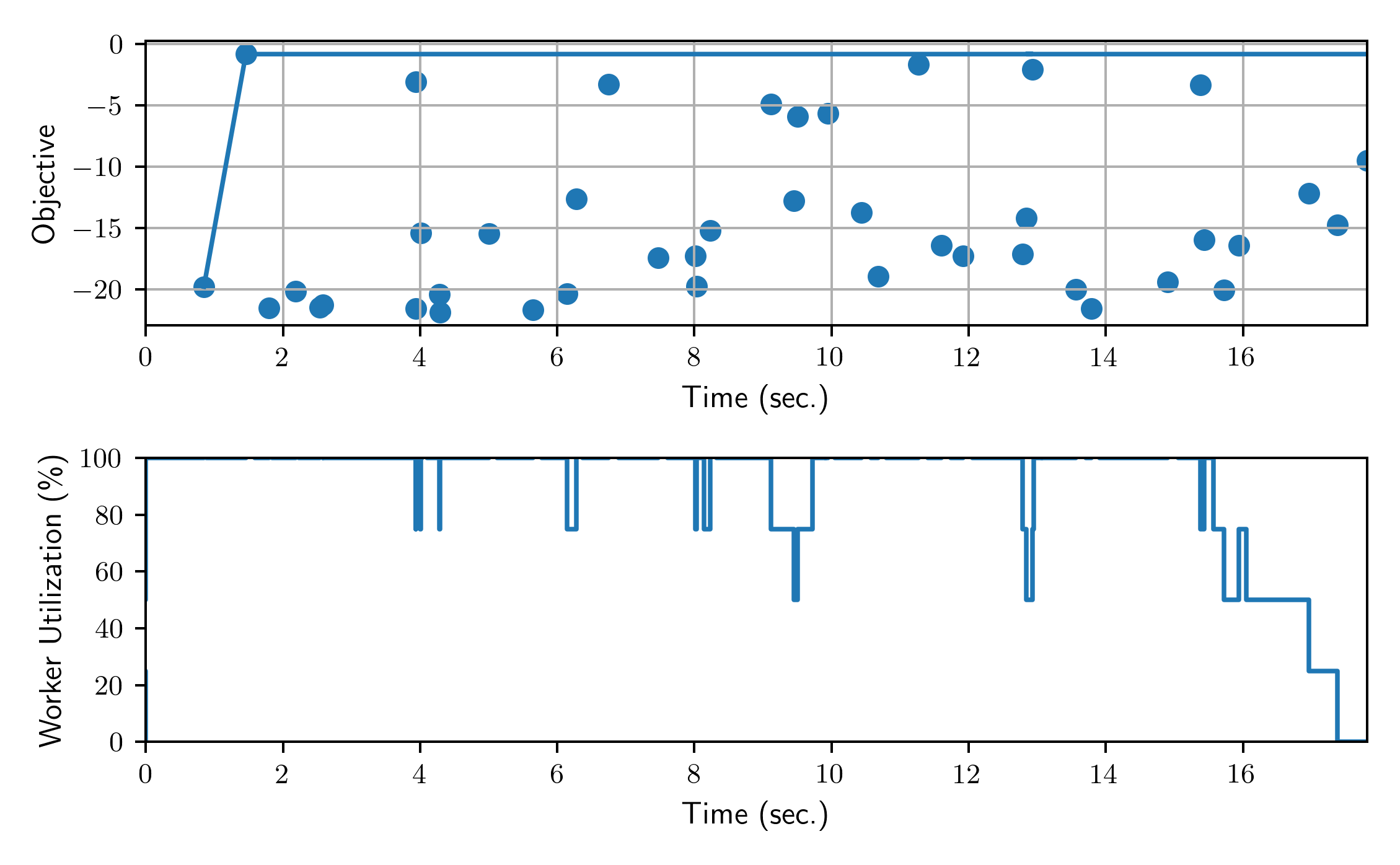
Finally, we plot the results from the collected DataFrame.
if __name__ == "__main__":
    import matplotlib.pyplot as plt
    import numpy as np

    def compile_profile(df):
        """Take the results dataframe as input and return the number of jobs running at a given timestamp."""
        history = []

        for _, row in df.iterrows():
            history.append((row["m:timestamp_start"], 1))
            history.append((row["m:timestamp_end"], -1))

        history = sorted(history, key=lambda v: v[0])
        nb_workers = 0
        timestamp = [0]
        n_jobs_running = [0]
        for time, incr in history:
            nb_workers += incr
            timestamp.append(time)
            n_jobs_running.append(nb_workers)

        return timestamp, n_jobs_running

    t0 = results["m:timestamp_start"].iloc[0]
    results["m:timestamp_start"] = results["m:timestamp_start"] - t0
    results["m:timestamp_end"] = results["m:timestamp_end"] - t0
    tmax = results["m:timestamp_end"].max()

    plt.figure()

    plt.subplot(2, 1, 1)
    plt.scatter(results["m:timestamp_end"], results.objective)
    plt.plot(results["m:timestamp_end"], results.objective.cummax())
    plt.xlabel("Time (sec.)")
    plt.ylabel("Objective")
    plt.grid()
    plt.xlim(0, tmax)

    plt.subplot(2, 1, 2)
    x, y = compile_profile(results)
    y = np.asarray(y) / num_workers * 100

    plt.step(
        x,
        y,
        where="pre",
    )
    plt.ylim(0, 100)
    plt.xlim(0, tmax)
    plt.xlabel("Time (sec.)")
    plt.ylabel("Worker Utilization (\%)")
    plt.tight_layout()
    plt.show()
Total running time of the script: (0 minutes 22.543 seconds)