1. Black-Box Single-Objective Optimiaztion with DeepHyper (Basic)

In this tutorial, we present the basics of DeepHyper.

Let us start with installing DeepHyper!

try:
    import deephyper
    print(deephyper.__version__)
except (ImportError, ModuleNotFoundError):
    !pip install deephyper

0.9.0

1.1. Optimization Problem

In the definition of our optimization problem we have two components:

1. black-box function that we want to optimize

2. the search space of input variables

1.1.1. Black-Box Function

DeepHyper is developed to optimize black-box functions. Here, we define the function \(f(x) = - x ^ 2\) that we want to maximise (the maximum being \(f(x=0) = 0\) on \(I_x = [-10;10]\)). The black-box function f takes as input a config dictionary from which we retrieve the variables of interest.

def f(job):
    return -job.parameters["x"] ** 2

1.1.2. Search Space of Input Variables

In this example, we have only one variable \(x\) for the black-box functin \(f\). We empirically decide to optimize this variable \(x\) on the interval \(I_x = [-10;10]\). To do so we use the HpProblem from DeepHyper and add a real hyperparameter by using a tuple of two floats.

from deephyper.hpo import HpProblem

problem = HpProblem()

# Define the variable you want to optimize
problem.add_hyperparameter((-10.0, 10.0), "x")

problem

Configuration space object:
  Hyperparameters:
    x, Type: UniformFloat, Range: [-10.0, 10.0], Default: 0.0

1.2. Evaluator Interface

DeepHyper uses an API called Evaluator to distribute the computation of black-box functions and adapt to different backends (e.g., threads, processes, MPI, Ray). An Evaluator object wraps the black-box function f that we want to optimize. Then a method parameter is used to select the backend and method_kwargs defines some available options of this backend.

Tip

The method="thread" provides parallel computation only if the black-box is releasing the global interpretor lock (GIL). Therefore, if you want parallelism in Jupyter notebooks you should use the Ray evaluator (method="ray") after installing Ray with pip install ray.

It is possible to define callbacks to extend the behaviour of Evaluator each time a function-evaluation is launched or completed. In this example we use the TqdmCallback to follow the completed evaluations and the evolution of the objective with a progress-bar.

from deephyper.evaluator import Evaluator
from deephyper.evaluator.callback import TqdmCallback


# define the evaluator to distribute the computation
evaluator = Evaluator.create(
    f,
    method="thread",
    method_kwargs={
        "num_workers": 4,
        "callbacks": [TqdmCallback()]
    },
)

print(f"Evaluator has {evaluator.num_workers} available worker{'' if evaluator.num_workers == 1 else 's'}")

Evaluator has 4 available workers

/Users/romainegele/Documents/Argonne/deephyper/src/deephyper/evaluator/_evaluator.py:148: UserWarning: Applying nest-asyncio patch for IPython Shell!
  warnings.warn("Applying nest-asyncio patch for IPython Shell!", category=UserWarning)

1.3. Search Algorithm

The next step is to define the search algorithm that we want to use. Here, we choose CBO (Centralized Bayesian Optimization) which is a sampling based Bayesian optimization strategy. This algorithm has the advantage of being asynchronous thanks to a constant liar strategy which is crutial to keep a good utilization of the resources when the number of available workers increases.

from deephyper.hpo import CBO

# define your search
search = CBO(
    problem,
    evaluator,
    acq_func="UCB",  # Acquisition function to Upper Confidence Bound
    multi_point_strategy="qUCB",  # Fast Multi-point strategy with q-Upper Confidence Bound
    n_jobs=2,  # Number of threads to fit surrogate models in parallel
)

WARNING:root:Results file already exists, it will be renamed to /Users/romainegele/Documents/Argonne/deephyper-tutorials/tutorials/colab/results_20241216-110109.csv

Then, we can execute the search for a given number of iterations by using the search.search(max_evals=...). It is also possible to use the timeout parameter if one needs a specific time budget (e.g., restricted computational time in machine learning competitions, allocation time in HPC).

results = search.search(max_evals=100)

Finally, let us visualize the results. The search(...) returns a DataFrame also saved locally under results.csv (in case of crash we don’t want to lose the possibly expensive evaluations already performed).

The DataFrame contains as columns:

1. the optimized hyperparameters: such as x in our case.

2. the objective maximised which directly match the results of the \(f\)-function in our example.

3. the job_id of each evaluated function (increased incrementally following the order of created evaluations).

4. the time of creation/collection of each task timestamp_submit and timestamp_gather respectively (in secondes, since the creation of the Evaluator).

results

	p:x	objective	job_id	job_status	m:timestamp_submit	m:timestamp_gather
0	-5.078683	-2.579302e+01	0	DONE	35.146809	35.147762
1	-2.815068	-7.924609e+00	3	DONE	35.146896	35.152473
2	-7.511938	-5.642921e+01	2	DONE	35.146888	35.152756
3	-1.459091	-2.128947e+00	1	DONE	35.146876	35.152964
4	-2.136483	-4.564558e+00	4	DONE	35.193908	35.194477
...	...	...	...	...	...	...
95	-0.000343	-1.177289e-07	92	DONE	45.278022	45.279034
96	0.000407	-1.654244e-07	96	DONE	45.793965	45.794279
97	0.000136	-1.862800e-08	97	DONE	45.793983	45.794650
98	0.000016	-2.482679e-10	98	DONE	45.793989	45.794811
99	-0.000914	-8.350525e-07	99	DONE	45.793993	45.794964

100 rows × 6 columns

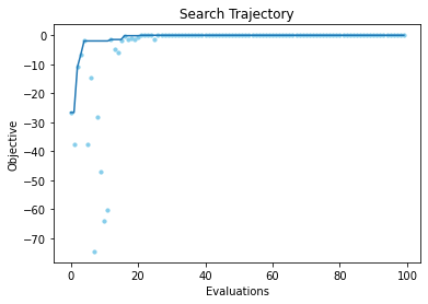
We can also plot the evolution of the objective to verify that we converge correctly toward \(0\).

import matplotlib.pyplot as plt
from deephyper.analysis.hpo import plot_search_trajectory_single_objective_hpo

fig, ax = plot_search_trajectory_single_objective_hpo(results, mode="min")
plt.title("Search Trajectory")
plt.yscale("log")
plt.show()