3. Understanding the pros and cons of Evaluator parallel backends

Author(s): Joceran Gouneau & Romain Egele.

In this tutorial we make an overview and comparison of all the evaluators available within DeepHyper.

3.1. The common base on which are tested the evaluators

3.1.1. The problem : the Ackley function with fixed duration

\[f(x) = -a \exp \left( -b \sqrt {\frac 1 d \sum_{i=1}^d x_i^2} \right) - \exp \left( -b \sqrt {\frac 1 d \sum_{i=1}^d \cos(c x_i)} \right) + a + \exp(1)\]

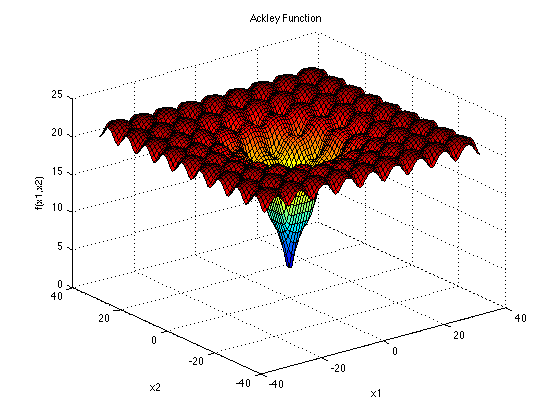
Let’s first define a common problem on which compare the evaluators ; for that we use the Ackley function as it emulates a complex problem while keeping the definition of the hyperparameter search space and run function very simple. Here we set \(d = 10\), \(a = 20\), \(b = 0.2\) and \(c = 2\pi\) and want to find its minimum \(f(x=(0, \dots , 0)) = 0\) on the domain \([-32.768, 32.768]^10\). Thus we define the hyperparameter problem as \(x_i \in [-32.768, 32.768]~ \forall i \in [|0,9|]\) and the objective returned by the run function as \(-f(x)\).

We also add a wait_function, to get closer to a classic use-case in which the black-box function usually isn’t as intantaneous as the evaluation of the Ackley function at a given point. We will always be using a simple basic_sleep function which only calls time.sleep(RUN_SLEEP), but in the case of the thread evaluator we will see that it is also usefull to make a distinction between a delay due to CPU or I/O communications limitations.

file: ackley.py

import time
import numpy as np
from deephyper.problem import HpProblem
from deephyper.evaluator import profile

d = 10
domain = (-32.768, 32.768)
hp_problem = HpProblem()
for i in range(d):
    hp_problem.add_hyperparameter(domain, f"x{i}")


def ackley(x, a=20, b=0.2, c=2 * np.pi):
    d = len(x)
    s1 = np.sum(x**2)
    s2 = np.sum(np.cos(c * x))
    term1 = -a * np.exp(-b * np.sqrt(s1 / d))
    term2 = -np.exp(s2 / d)
    y = term1 + term2 + a + np.exp(1)
    return y


from common import RUN_SLEEP


def basic_sleep():
    time.sleep(RUN_SLEEP)


def cpu_bound():
    t = time.time()
    duration = 0
    while duration < RUN_SLEEP:
        sum(i * i for i in range(10**7))
        duration = time.time() - t


def IO_bound():
    with open("/dev/urandom", "rb") as f:
        t = time.time()
        duration = 0
        while duration < RUN_SLEEP:
            f.read(100)
            duration = time.time() - t


wait_functions = dict(
    basic_sleep=basic_sleep,
    cpu_bound=cpu_bound,
    IO_bound=IO_bound,
)


@profile
def run(config, wait_function="basic_sleep"):
    #! wait_function
    wait_functions.get(wait_function)()

    #! real function
    x = np.array([config[f"x{i}"] for i in range(d)])
    x = np.asarray_chkfinite(x)  # ValueError if any NaN or Inf
    return -ackley(x)

Note

We decorate the run-function with @profile to collect exact run-times of the run-function referenced as timestamp_start and timestamp_end in the results.

3.1.2. The search algorithm : as quick as possible

We define a simple search receiving the chosen evaluator as well as the hp_problem defined in ackley.py.

Warning

DUMMY is a surrogate model performing random search, meaning there is no time lost in fitting a model to the new evaluations. The parameter filter_duplicated=False makes it possible to re-generate already evaluated configurations, thus saving the time of of checking for duplicated configurations. These choices were made to minimize as much as possible the overheads of search algorithm (reduce the amount of mixed effects) in order to better highlight the overhead due to the choice of Evaluator.

search = CBO(
     hp_problem,
     evaluator,
     surrogate_model="DUMMY",
     filter_duplicated=False
 )

 results = search.search(timeout=SEARCH_TIMEOUT)
 results.to_csv("results.csv")

This search instance is defined along with the functions used to evaluate the performances and plot the insights of an evaluator’s execution in a common.py python script :

file: common.py

import pathlib
import time
import pandas as pd
import matplotlib.pyplot as plt
import matplotlib.ticker as ticker

from deephyper.search.hps import CBO
from ackley import hp_problem

NUM_WORKERS = 5
SEARCH_TIMEOUT = 20
RUN_SLEEP = 1


def execute_search(evaluator):
    t = time.time()
    init_duration = t - evaluator.timestamp
    evaluator.timestamp = t

    search = CBO(
        hp_problem, evaluator, surrogate_model="DUMMY", filter_duplicated=False
    )

    results = search.search(timeout=SEARCH_TIMEOUT)
    results.to_csv("results.csv")

    return init_duration


def get_profile_from_hist(hist):
    n_processes = 0
    profile_dict = dict(t=[0], n_processes=[0])
    for e in sorted(hist):
        t, incr = e
        n_processes += incr
        profile_dict["t"].append(t)
        profile_dict["n_processes"].append(n_processes)
    profile = pd.DataFrame(profile_dict)
    return profile


def get_perc_util(profile):
    csum = 0
    for i in range(len(profile) - 1):
        csum += (profile.loc[i + 1, "t"] - profile.loc[i, "t"]) * profile.loc[
            i, "n_processes"
        ]
    perc_util = csum / (profile["t"].iloc[-1] * 6)
    return perc_util


def plot_profile(ax, profile, ylabel="None", color="blue"):
    ax.step(profile["t"], profile["n_processes"], where="post", color=color)
    ax.set_ylabel(ylabel)
    ax.set_ylim(0, NUM_WORKERS + 1)
    ax.yaxis.set_major_locator(ticker.MultipleLocator(1))
    ax.grid()


def plot_sum_up(name, init_duration):

    pathlib.Path("plots").mkdir(parents=False, exist_ok=True)
    results = pd.read_csv("results.csv")

    # compute profiles from results.csv
    jobs_hist = []
    runs_hist = []
    for _, row in results.iterrows():
        jobs_hist.append((row["timestamp_submit"], 1))
        jobs_hist.append((row["timestamp_gather"], -1))
        runs_hist.append((row["timestamp_start"], 1))
        runs_hist.append((row["timestamp_end"], -1))

    jobs_profile = get_profile_from_hist(jobs_hist)
    runs_profile = get_profile_from_hist(runs_hist)

    # compute average job and run durations
    job_avrg_duration = (
        results["timestamp_gather"] - results["timestamp_submit"]
    ).mean()

    # compute perc_util
    jobs_perc_util = get_perc_util(jobs_profile)
    runs_perc_util = get_perc_util(runs_profile)

    # compute total number of evaluations
    total_num_eval = len(results)

    # plot
    fig, axs = plt.subplots(2, sharex=True)
    fig.suptitle(name, fontsize=17)
    plot_profile(axs[0], jobs_profile, ylabel="# jobs submitted", color="blue")
    plot_profile(axs[1], runs_profile, ylabel="# jobs running", color="crimson")
    fig.text(0.1, -0.1, f"init_duration: {init_duration:.2f}s.", fontsize=12)
    fig.text(0.1, -0.2, f"job_avrg_duration: {job_avrg_duration:.2f}s.", fontsize=12)
    fig.text(0.1, -0.3, f"total_num_eval: {total_num_eval}", fontsize=12)
    fig.text(
        0.6,
        -0.1,
        f"jobs_perc_util: {100*jobs_perc_util:.1f}%",
        fontsize=12,
        color="blue",
    )
    fig.text(
        0.6,
        -0.2,
        f"runs_perc_util: {100*runs_perc_util:.1f}%",
        fontsize=12,
        color="crimson",
    )
    fig.tight_layout()
    plt.savefig(f"plots/{name}.jpg", bbox_inches="tight")


def evaluate_and_plot(evaluator, name):

    init_duration = execute_search(evaluator)

    plot_sum_up(name, init_duration)

3.1.3. The output : profile plots and insights

To execute a certain evaluator, you just have to run :

python evaluator_{type}.py

Except for MPI, which execution depends on your machine and your installation. This will generate a “profile” plot in the plots/ directory such as:

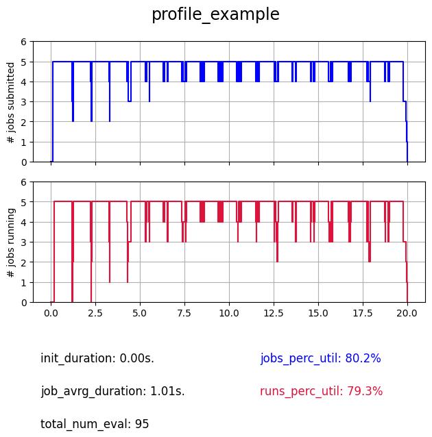
where - the top plot represents the number of submitted jobs (which means waiting for execution or being executed), it represents the state of the evaluator and how it manages these jobs. - the bottom plot represents the number of simultaneously running jobs (jobs being executed), it represents the state of the workers and the true usage of allocated ressources (here NUM_WORKERS=5). - init_duration: the duration of the initialization. - job_avrg_duration: the jobs average duration (from submission to collection, in other words run_duration + evaluator_overhead with RUN_SLEEP=1 in ackley.py). - total_num_eval: the total number of evaluations within the budget of 20 secondes for the search (SEARCH_TIMEOUT=20). - two percentage of utilization (for each profile) corresponding to each profile (jobs_perc_util for the top plot and runs_perc_util for the bottom plot). It is the area under the respective curves normalized by the theorical optimal case (maximal number of workers during the whole search, which is NUM_WORKERS * SEARCH_TIMEOUT).

3.2. Serial

file: evaluator_serial.py

if __name__ == "__main__":
    from deephyper.evaluator import Evaluator
    from ackley import run
    from common import NUM_WORKERS, evaluate_and_plot

    evaluator = Evaluator.create(
        run,
        method="serial",
        method_kwargs=dict(
            num_workers=NUM_WORKERS,
        ),
    )

    evaluate_and_plot(evaluator, "serial_evaluator")

The serial evaluator is the most basic, it is a single thread based evaluator, which means that whatever the number of workers it is given, it will always perform its evaluations sequentialy on one worker.

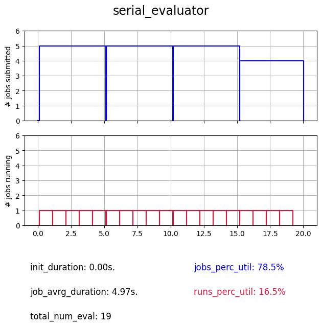
As we can see despite the fact that it is always submitting NUM_WORKERS jobs, in reality there is only one evaluation performed at a time, thus resulting in poor utilization of the computational ressources.

Note

This evaluator is practicaly useful when debugging because everything is happening in the same Python thread.

Warning

It is important to notice the if __name__ == "__main__": statement at the beginning of the script. Not all evaluators require it but it is a good practice to use it. Some evaluators will initialize new processes, potentially reloading the main script which could trigger a recursive infinite reloading of modules. Adding this statement avoids this type of issue.

3.3. Thread

file: evaluator_thread.py

if __name__ == "__main__":
    from deephyper.evaluator import Evaluator
    from ackley import run
    from common import NUM_WORKERS, evaluate_and_plot

    wait_function = "cpu_bound"  # or "IO_bound"

    evaluator = Evaluator.create(
        run,
        method="thread",
        method_kwargs=dict(
            num_workers=NUM_WORKERS,
            run_function_kwargs={"wait_function": wait_function},
        ),
    )

    evaluate_and_plot(evaluator, f"thread_evaluator_{wait_function}")

The thread evaluator is using the ThreadPoolExecutor backend. Therefore it has access to multiple Python threads (but Python is single threaded due to the global lock interpreter) and becomes usefull especially when I/O-bound computation is involved, as it can take advantages of these wait times switch to other threads and have a concurrent execution.

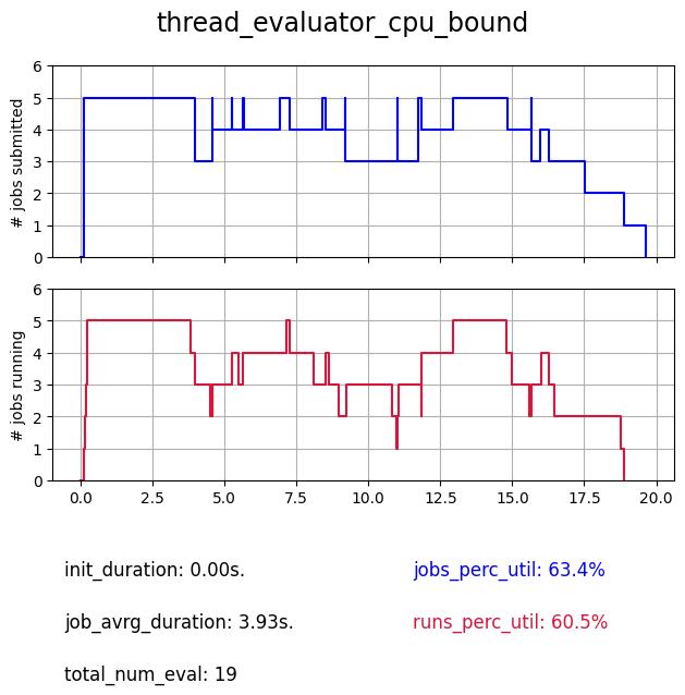
As we can see when computation is involved the profile is not maximized. But we expect a better utilization in case of I/O-bound functions which we illustrate bellow.:

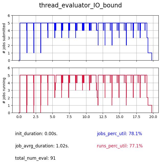
The advantage of the thread evaluator on I/O communications is clear with 91 evaluations performed instead of 19.

3.4. Process

file: evaluator_process.py

if __name__ == "__main__":
    from deephyper.evaluator import Evaluator
    from ackley import run
    from common import NUM_WORKERS, evaluate_and_plot

    evaluator = Evaluator.create(
        run,
        method="process",
        method_kwargs=dict(
            num_workers=NUM_WORKERS,
        ),
    )

    evaluate_and_plot(evaluator, "process_evaluator")

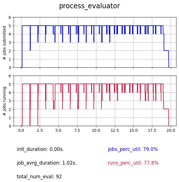
Then the process based evaluator is a better choice for cpu-bound functions. It also avoid repetitive overheads due to initialization of processes because the pool of processes is instanciated once and re-used.

3.5. Subprocess

file: evaluator_subprocess.py

if __name__ == "__main__":
    from deephyper.evaluator import Evaluator
    from ackley import run
    from common import NUM_WORKERS, evaluate_and_plot

    evaluator = Evaluator.create(
        run,
        method="subprocess",
        method_kwargs=dict(
            num_workers=NUM_WORKERS,
        ),
    )

    evaluate_and_plot(evaluator, "subprocess_evaluator")

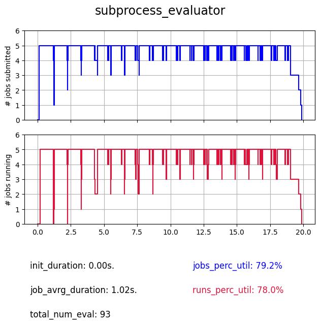
The subprocess evaluator is similar to process but it creates new processes from scratch each time, it can be practicle in some cases to aleviate the limiates of process evaluator.

3.6. Ray

file: evaluator_ray.py

if __name__ == "__main__":
    from deephyper.evaluator import Evaluator
    from ackley import run
    from common import NUM_WORKERS, evaluate_and_plot

    evaluator = Evaluator.create(
        run,
        method="ray",
        method_kwargs=dict(
            num_workers=NUM_WORKERS,
        ),
    )

    evaluate_and_plot(evaluator, "ray_evaluator")

The Ray evaluator uses the ray library as backend, its advantage comes from the fact that once ray workers are instanciated they are not stopped till the end of the search, which means that once an import is made it doesn’t have to be re-performed at each evaluation, which can save a lot of time on certain tasks. The major drawback is that this setup requires an initialization of the Ray-cluster which can take time and be complex and source of issues on very large systems.

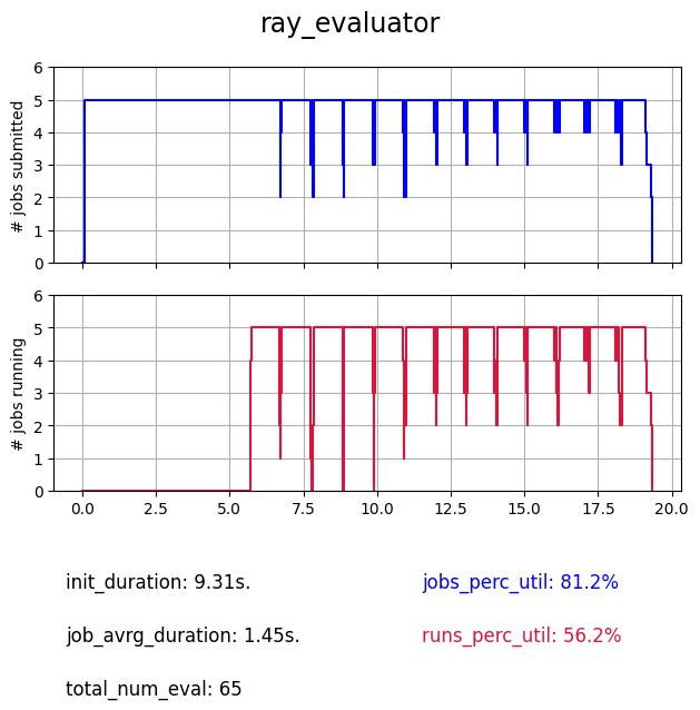
As we can see the initialization takes here (on a simple system with 6 cores) around 9s., and there is also an overhead of 5s. happening at the beggining of the search for initializing the communications. But once it is started it is as concistent as process and subprocess, and can keep it up with more workers.

3.7. MPI

file: evaluator_mpi.py

if __name__ == "__main__":
    from deephyper.evaluator import Evaluator
    from ackley import run
    from common import evaluate_and_plot

    with Evaluator.create(
        run,
        method="mpicomm",
    ) as evaluator:
        if evaluator is not None:
            evaluate_and_plot(evaluator, "mpi_evaluator")

The MPI evaluator uses the mpi4py library as backend, like the Ray evaluator imports are done once and not re-performed at each evaluation, to execute it you need an MPI instance your machine, which is common on big systems thus making it the most convenient choice to perform searches at scale.

This has to be executed with MPI such as:

$ mpirun -np 6 python evaluator_mpi.py

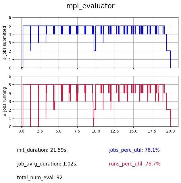
Like the Ray evaluator, there is an initialization taking here around 20s., but once launched there is very few overhead. Also this initialization step can be optimized depending on the local MPI implementation. For example in our case we use:

import mpi4py

mpi4py.rc.initialize = False
mpi4py.rc.threads = True
mpi4py.rc.thread_level = "multiple"