3. Multi-Fidelity Hyperparameter Optimiaztion for Classification with Tabular Data (Tensorflow/Keras2)

In this tutorial we present how to use hyperparameter optimization on an example from the Keras documentation. We follow the previous tutorial based on the same example and add multi-fidelity to it. The purpose of multi-fidelity is to dynamically manage the budget allocated (also called fidelity) to evaluate an hyperparameter configuration. For example, when training a deep neural network the number of epochs can be continued or stopped based on currently observed performance and some policy.

In DeepHyper, the multi-fidelity agent is designed separately from the hyperparameter search agent. Of course, both can communicate but from an API perspective they are different objects. The multi-fidelity agents are called Stopper in DeepHyper and their documentation can be found at deephyper.stopper.

In this notebook, we will demonstrate how to use multi-fidelity inside sequential Bayesian optimization. When moving to a distributed setting, it is important to use a shared memory accessible by all workers otherwise the multi-fidelity scheme may not work properly. An example, of database instanciation for parallel computing is explained in: Introduction to Distributed Bayesian Optimization (DBO) with MPI (Communication) and Redis (Storage).

Reference: This tutorial is based on materials from the Keras Documentation: Structured data classification from scratch

Let us start with installing DeepHyper!

Warning

Since the release of Keras 3.0, this tutorial should be run with tf-keras (link to pypi).

try:
    import deephyper
    import deephyper.stopper.lce
except (ImportError, ModuleNotFoundError):
    !pip install "deephyper[tf-keras2,jax-cpu]"
    import deephyper
    import deephyper.stopper.lce
print(deephyper.__version__)

0.9.0

Note

The following environment variables can be used to avoid the logging of some Tensorflow DEBUG, INFO and WARNING statements.

import os

os.environ["TF_CPP_MIN_LOG_LEVEL"] = str(4)
os.environ["AUTOGRAPH_VERBOSITY"] = str(0)

3.1. Imports

import pandas as pd
import tensorflow as tf
import tf_keras as tfk
tf.get_logger().setLevel("ERROR")

3.2. The dataset (from Keras.io)

The dataset is provided by the Cleveland Clinic Foundation for Heart Disease. It’s a CSV file with 303 rows. Each row contains information about a patient (a sample), and each column describes an attribute of the patient (a feature). We use the features to predict whether a patient has a heart disease (binary classification).

Here’s the description of each feature:

Column	Description	Feature Type
Age	Age in years	Numerical
Sex	(1 = male; 0 = female)	Categorical
CP	Chest pain type (0, 1, 2, 3, 4)	Categorical
Trestbpd	Resting blood pressure (in mm Hg on admission)	Numerical
Chol	Serum cholesterol in mg/dl	Numerical
FBS	fasting blood sugar in 120 mg/dl (1 = true; 0 = false)	Categorical
RestECG	Resting electrocardiogram results (0, 1, 2)	Categorical
Thalach	Maximum heart rate achieved	Numerical
Exang	Exercise induced angina (1 = yes; 0 = no)	Categorical
Oldpeak	ST depression induced by exercise relative to rest	Numerical
Slope	Slope of the peak exercise ST segment	Numerical
CA	Number of major vessels (0-3) colored by fluoroscopy	Both numerical & categorical
Thal	3 = normal; 6 = fixed defect; 7 = reversible defect	Categorical
Target	Diagnosis of heart disease (1 = true; 0 = false)	Target

def load_data():
    file_url = "http://storage.googleapis.com/download.tensorflow.org/data/heart.csv"
    dataframe = pd.read_csv(file_url)

    val_dataframe = dataframe.sample(frac=0.2, random_state=1337)
    train_dataframe = dataframe.drop(val_dataframe.index)

    return train_dataframe, val_dataframe


def dataframe_to_dataset(dataframe):
    dataframe = dataframe.copy()
    labels = dataframe.pop("target")
    ds = tf.data.Dataset.from_tensor_slices((dict(dataframe), labels))
    ds = ds.shuffle(buffer_size=len(dataframe))
    return ds

3.3. Preprocessing & encoding of features

The next cells use tfk.layers.Normalization() to apply standard scaling on the features.

Then, the tfk.layers.StringLookup and tfk.layers.IntegerLookup are used to encode categorical variables.

def encode_numerical_feature(feature, name, dataset):
    # Create a Normalization layer for our feature
    normalizer = tfk.layers.Normalization()

    # Prepare a Dataset that only yields our feature
    feature_ds = dataset.map(lambda x, y: x[name])
    feature_ds = feature_ds.map(lambda x: tf.expand_dims(x, -1))

    # Learn the statistics of the data
    normalizer.adapt(feature_ds)

    # Normalize the input feature
    encoded_feature = normalizer(feature)
    return encoded_feature


def encode_categorical_feature(feature, name, dataset, is_string):
    lookup_class = (
        tfk.layers.StringLookup if is_string else tfk.layers.IntegerLookup
    )
    # Create a lookup layer which will turn strings into integer indices
    lookup = lookup_class(output_mode="binary")

    # Prepare a Dataset that only yields our feature
    feature_ds = dataset.map(lambda x, y: x[name])
    feature_ds = feature_ds.map(lambda x: tf.expand_dims(x, -1))

    # Learn the set of possible string values and assign them a fixed integer index
    lookup.adapt(feature_ds)

    # Turn the string input into integer indices
    encoded_feature = lookup(feature)
    return encoded_feature

3.4. Define the run-function with multi-fidelity

The run-function defines how the objective that we want to maximize is computed. It takes a job (see deephyper.evaluator.RunningJob) as input and outputs a scaler value or dictionnary (see deephyper.evaluator). The objective is always maximized in DeepHyper. The job.parameters contains a suggested configuration of hyperparameters that we want to evaluate. In this example we will search for:

• units (default value: 32)

• activation (default value: "relu")

• dropout_rate (default value: 0.5)

• batch_size (default value: 32)

• learning_rate (default value: 1e-3)

A hyperparameter value can be acessed easily in the dictionary through the corresponding key, for example job["units"] or job.parameters["units"] are both valid. Unlike the previous tutorial in this example we want to use multi-fidelity to dynamically choose the allocated budget of each evaluation. Therefore we use the tensorflow keras integration of stoppers deephyper.stopper.integration.TFKerasStopperCallback. The multi-fidelity agent will monitor the validation accuracy (val_accuracy) in the context of maximization. This stopper_callback is then added to the callbacks used by the model during the training. In order to collect more information about the execution of our job we use the @profile decorator on the run-function which will collect execution timings (timestamp_start and timestamp_end). We will also add "metadata" to the output of our function to know how many epochs were used to evaluate each model. To learn more about how the @profile decorator can be used check our tutorial on Understanding the pros and cons of Evaluator parallel backends.

stopper_callback = TFKerasStopperCallback(
    job,
    monitor="val_accuracy",
    mode="max"
)

history = model.fit(
    train_ds,
    epochs=100,
    validation_data=val_ds,
    verbose=0,
    callbacks=[stopper_callback]
)


objective = history.history["val_accuracy"][-1]
metadata = {"budget": stopper_callback.budget}
return {"objective": objective, "metadata": metadata}

import json

from deephyper.evaluator import profile, RunningJob
from deephyper.stopper.integration.tf_keras2 import TFKerasStopperCallback


@profile
def run(job: RunningJob):

    config = job.parameters

    def create_and_fit_model():
        tf.autograph.set_verbosity(0)
        import absl.logging
        absl.logging.set_verbosity(absl.logging.ERROR)

        # Load data and split into validation set
        train_dataframe, val_dataframe = load_data()
        train_ds = dataframe_to_dataset(train_dataframe)
        val_ds = dataframe_to_dataset(val_dataframe)
        train_ds = train_ds.batch(config["batch_size"])
        val_ds = val_ds.batch(config["batch_size"])

        # Categorical features encoded as integers
        sex = tfk.Input(shape=(1,), name="sex", dtype="int64")
        cp = tfk.Input(shape=(1,), name="cp", dtype="int64")
        fbs = tfk.Input(shape=(1,), name="fbs", dtype="int64")
        restecg = tfk.Input(shape=(1,), name="restecg", dtype="int64")
        exang = tfk.Input(shape=(1,), name="exang", dtype="int64")
        ca = tfk.Input(shape=(1,), name="ca", dtype="int64")

        # Categorical feature encoded as string
        thal = tfk.Input(shape=(1,), name="thal", dtype="string")

        # Numerical features
        age = tfk.Input(shape=(1,), name="age")
        trestbps = tfk.Input(shape=(1,), name="trestbps")
        chol = tfk.Input(shape=(1,), name="chol")
        thalach = tfk.Input(shape=(1,), name="thalach")
        oldpeak = tfk.Input(shape=(1,), name="oldpeak")
        slope = tfk.Input(shape=(1,), name="slope")

        all_inputs = [
            sex,
            cp,
            fbs,
            restecg,
            exang,
            ca,
            thal,
            age,
            trestbps,
            chol,
            thalach,
            oldpeak,
            slope,
        ]

        # Integer categorical features
        sex_encoded = encode_categorical_feature(sex, "sex", train_ds, False)
        cp_encoded = encode_categorical_feature(cp, "cp", train_ds, False)
        fbs_encoded = encode_categorical_feature(fbs, "fbs", train_ds, False)
        restecg_encoded = encode_categorical_feature(restecg, "restecg", train_ds, False)
        exang_encoded = encode_categorical_feature(exang, "exang", train_ds, False)
        ca_encoded = encode_categorical_feature(ca, "ca", train_ds, False)

        # String categorical features
        thal_encoded = encode_categorical_feature(thal, "thal", train_ds, True)

        # Numerical features
        age_encoded = encode_numerical_feature(age, "age", train_ds)
        trestbps_encoded = encode_numerical_feature(trestbps, "trestbps", train_ds)
        chol_encoded = encode_numerical_feature(chol, "chol", train_ds)
        thalach_encoded = encode_numerical_feature(thalach, "thalach", train_ds)
        oldpeak_encoded = encode_numerical_feature(oldpeak, "oldpeak", train_ds)
        slope_encoded = encode_numerical_feature(slope, "slope", train_ds)

        all_features = tfk.layers.concatenate(
            [
                sex_encoded,
                cp_encoded,
                fbs_encoded,
                restecg_encoded,
                exang_encoded,
                slope_encoded,
                ca_encoded,
                thal_encoded,
                age_encoded,
                trestbps_encoded,
                chol_encoded,
                thalach_encoded,
                oldpeak_encoded,
            ]
        )
        x = tfk.layers.Dense(config["units"], activation=config["activation"])(
            all_features
        )
        x = tfk.layers.Dropout(config["dropout_rate"])(x)
        output = tfk.layers.Dense(1, activation="sigmoid")(x)
        model = tfk.Model(all_inputs, output)

        optimizer = tfk.optimizers.Adam(learning_rate=config["learning_rate"])
        model.compile(optimizer, "binary_crossentropy", metrics=["accuracy"])

        stopper_callback = TFKerasStopperCallback(
            job,
            monitor="val_accuracy",
            mode="max"
        )

        history = model.fit(
                train_ds,
                epochs=100,
                validation_data=val_ds,
                verbose=0,
                callbacks=[stopper_callback]
            )
        return history, stopper_callback.budget

    try:
        history, budget = create_and_fit_model()
    except:
        class History:
            history = {
                "accuracy": None,
                "val_accuracy": ["F_fit"],
                "loss": None,
                "val_loss": None,
            }

        history, budget = History(), 0


    objective = history.history["val_accuracy"][-1]
    metadata = {
        "loss": history.history["loss"],
        "val_loss": history.history["val_loss"],
        "accuracy": history.history["accuracy"],
        "val_accuracy": history.history["val_accuracy"],
    }
    metadata = {k:json.dumps(v) for k,v in metadata.items()}
    metadata["budget"] = budget
    return {"objective": objective, "metadata": metadata}

Note

The objective maximized by DeepHyper is the "objective" value returned by the run-function.

In this tutorial it corresponds to the validation accuracy of the last epoch of training which we retrieve in the History object returned by the model.fit(...) call.

...
objective = history.history["val_accuracy"][-1]
...

Using an objective like max(history.history['val_accuracy']) can have undesired side effects.

For example, it is possible that the training curves will overshoot a local maximum, resulting in a model without the capacity to flexibly adapt to new data in the future.

3.5. Define the Hyperparameter optimization problem

Hyperparameter ranges are defined using the following syntax:

• Discrete integer ranges are generated from a tuple (lower: int, upper: int)

• Continuous prarameters are generated from a tuple (lower: float, upper: float)

• Categorical or nonordinal hyperparameter ranges can be given as a list of possible values [val1, val2, ...]

from deephyper.hpo import HpProblem


# Creation of an hyperparameter problem
problem = HpProblem()

# Discrete hyperparameter (sampled with uniform prior)
problem.add_hyperparameter((8, 128), "units", default_value=32)


# Categorical hyperparameter (sampled with uniform prior)
ACTIVATIONS = [
    "elu", "gelu", "hard_sigmoid", "linear", "relu", "selu",
    "sigmoid", "softplus", "softsign", "swish", "tanh",
]
problem.add_hyperparameter(ACTIVATIONS, "activation", default_value="relu")


# Real hyperparameter (sampled with uniform prior)
problem.add_hyperparameter((0.0, 0.6), "dropout_rate", default_value=0.5)


# Discrete and Real hyperparameters (sampled with log-uniform)
problem.add_hyperparameter((8, 256, "log-uniform"), "batch_size", default_value=32)
problem.add_hyperparameter((1e-5, 1e-2, "log-uniform"), "learning_rate", default_value=1e-3)

problem

Configuration space object:
  Hyperparameters:
    activation, Type: Categorical, Choices: {elu, gelu, hard_sigmoid, linear, relu, selu, sigmoid, softplus, softsign, swish, tanh}, Default: relu
    batch_size, Type: UniformInteger, Range: [8, 256], Default: 32, on log-scale
    dropout_rate, Type: UniformFloat, Range: [0.0, 0.6], Default: 0.5
    learning_rate, Type: UniformFloat, Range: [1e-05, 0.01], Default: 0.001, on log-scale
    units, Type: UniformInteger, Range: [8, 128], Default: 32

3.6. Evaluate a default configuration

We evaluate the performance of the default set of hyperparameters provided in the Keras tutorial.

out = run(RunningJob(parameters=problem.default_configuration))

objective_default = out["output"]["objective"]
metadata_default = out["metadata"].copy()
metadata_default.update(out["output"]["metadata"])

print(f"Accuracy of the default configuration is {objective_default:.3f} with a budget of {metadata_default['budget']} epochs.")

out

Accuracy of the default configuration is 0.787 with a budget of 100 epochs.

{'output': {'objective': 0.7868852615356445,
  'metadata': {'loss': '[0.8586015105247498, 0.7996073365211487, 0.7143529653549194, 0.7026970982551575, 0.6131916046142578, 0.5995704531669617, 0.5482029318809509, 0.5406618714332581, 0.5241131782531738, 0.524106502532959, 0.49953699111938477, 0.48616209626197815, 0.4766983389854431, 0.4396292269229889, 0.42282265424728394, 0.4252450466156006, 0.42260438203811646, 0.40739893913269043, 0.38850900530815125, 0.39543795585632324, 0.38968002796173096, 0.3746700584888458, 0.3902652859687805, 0.34748750925064087, 0.3520696759223938, 0.37348535656929016, 0.3489677906036377, 0.3853694796562195, 0.3613702654838562, 0.34566059708595276, 0.32275688648223877, 0.2991926074028015, 0.32832810282707214, 0.3174874782562256, 0.3352506458759308, 0.31052303314208984, 0.3016624450683594, 0.3174218535423279, 0.3001049757003784, 0.320993036031723, 0.30082637071609497, 0.30680087208747864, 0.31447672843933105, 0.28569477796554565, 0.29206568002700806, 0.31954723596572876, 0.32253536581993103, 0.30184730887413025, 0.3012655973434448, 0.2885284721851349, 0.2924761474132538, 0.27612340450286865, 0.28211188316345215, 0.27235496044158936, 0.28846436738967896, 0.29557710886001587, 0.2503412067890167, 0.27671802043914795, 0.2697695791721344, 0.270313024520874, 0.27802953124046326, 0.2447458654642105, 0.27979663014411926, 0.24681539833545685, 0.23311007022857666, 0.24984775483608246, 0.2718290090560913, 0.25780507922172546, 0.2598930597305298, 0.24725821614265442, 0.25572851300239563, 0.25640401244163513, 0.2774571478366852, 0.25011134147644043, 0.25798243284225464, 0.23662544786930084, 0.23648932576179504, 0.2736731469631195, 0.2540879547595978, 0.2552516758441925, 0.27141138911247253, 0.25138428807258606, 0.24117296934127808, 0.24266380071640015, 0.2398163378238678, 0.24061521887779236, 0.2434554100036621, 0.25063556432724, 0.24322843551635742, 0.241098552942276, 0.23228313028812408, 0.23064105212688446, 0.23888643085956573, 0.2367614358663559, 0.22047720849514008, 0.2215237319469452, 0.21931636333465576, 0.24564103782176971, 0.2615945637226105, 0.21107320487499237]',
   'val_loss': '[0.7731939554214478, 0.7041282653808594, 0.6490469574928284, 0.6033157706260681, 0.566530704498291, 0.5350698232650757, 0.5093625783920288, 0.48751768469810486, 0.47036299109458923, 0.45570504665374756, 0.44297927618026733, 0.4324043095111847, 0.42428669333457947, 0.41646507382392883, 0.4094529449939728, 0.4042246341705322, 0.3995428681373596, 0.3959790766239166, 0.3934732675552368, 0.39177680015563965, 0.39164412021636963, 0.3913073241710663, 0.38937148451805115, 0.3881676495075226, 0.38752859830856323, 0.3878481984138489, 0.3882769048213959, 0.3893079459667206, 0.39045751094818115, 0.38898178935050964, 0.3874622583389282, 0.38792648911476135, 0.3885522484779358, 0.3897016644477844, 0.3899131417274475, 0.3892446458339691, 0.3893031179904938, 0.39050817489624023, 0.3913511037826538, 0.39246517419815063, 0.39239686727523804, 0.39178910851478577, 0.3916884958744049, 0.3904183804988861, 0.38918906450271606, 0.38943561911582947, 0.3889676630496979, 0.38773661851882935, 0.38719406723976135, 0.3878912031650543, 0.3887121081352234, 0.3896653354167938, 0.3893643915653229, 0.39059385657310486, 0.3905489444732666, 0.39046376943588257, 0.390889972448349, 0.3924510180950165, 0.3930373191833496, 0.3926296532154083, 0.3929689824581146, 0.3926841616630554, 0.39288032054901123, 0.39369523525238037, 0.3942595422267914, 0.39491453766822815, 0.3940185308456421, 0.3942662477493286, 0.39511701464653015, 0.3963031470775604, 0.39753109216690063, 0.39771392941474915, 0.3972932994365692, 0.3978917896747589, 0.39735597372055054, 0.39732155203819275, 0.3984433710575104, 0.39892396330833435, 0.39780914783477783, 0.3956872820854187, 0.3948351740837097, 0.3936671316623688, 0.39478129148483276, 0.3951336145401001, 0.3958606421947479, 0.3964930772781372, 0.3961707651615143, 0.3955737054347992, 0.3949708342552185, 0.3943345844745636, 0.39364561438560486, 0.39376264810562134, 0.3939083218574524, 0.3955366909503937, 0.39585644006729126, 0.3969064950942993, 0.3977656364440918, 0.3982703387737274, 0.39910033345222473, 0.3997335731983185]',
   'accuracy': '[0.40082645416259766, 0.4628099203109741, 0.5454545617103577, 0.5330578684806824, 0.6404958963394165, 0.6611570119857788, 0.7479338645935059, 0.7355371713638306, 0.7355371713638306, 0.7355371713638306, 0.7479338645935059, 0.7809917330741882, 0.8140496015548706, 0.797520637512207, 0.78925621509552, 0.8181818127632141, 0.8099173307418823, 0.8223140239715576, 0.8388429880142212, 0.8264462947845459, 0.8016529083251953, 0.8305785059928894, 0.8429751992225647, 0.8512396812438965, 0.85537189245224, 0.8305785059928894, 0.8636363744735718, 0.8305785059928894, 0.8429751992225647, 0.8429751992225647, 0.8760330677032471, 0.8719007968902588, 0.8595041036605835, 0.8760330677032471, 0.8636363744735718, 0.8636363744735718, 0.8595041036605835, 0.8512396812438965, 0.8719007968902588, 0.8471074104309082, 0.8801652789115906, 0.8719007968902588, 0.8636363744735718, 0.8801652789115906, 0.8595041036605835, 0.85537189245224, 0.8636363744735718, 0.8760330677032471, 0.8636363744735718, 0.8801652789115906, 0.8801652789115906, 0.8760330677032471, 0.8719007968902588, 0.8801652789115906, 0.8636363744735718, 0.8801652789115906, 0.9173553586006165, 0.8884297609329224, 0.8636363744735718, 0.8842975497245789, 0.8966942429542542, 0.8842975497245789, 0.8842975497245789, 0.8925619721412659, 0.9049586653709412, 0.8884297609329224, 0.8760330677032471, 0.8884297609329224, 0.8966942429542542, 0.8842975497245789, 0.8760330677032471, 0.8842975497245789, 0.8719007968902588, 0.8884297609329224, 0.8966942429542542, 0.8966942429542542, 0.9173553586006165, 0.8842975497245789, 0.8884297609329224, 0.9049586653709412, 0.8595041036605835, 0.9090909361839294, 0.9173553586006165, 0.8925619721412659, 0.8966942429542542, 0.9049586653709412, 0.8760330677032471, 0.8925619721412659, 0.8925619721412659, 0.9049586653709412, 0.8884297609329224, 0.9049586653709412, 0.8925619721412659, 0.8925619721412659, 0.9214876294136047, 0.8966942429542542, 0.9049586653709412, 0.8884297609329224, 0.9008264541625977, 0.9173553586006165]',
   'val_accuracy': '[0.31147539615631104, 0.5081967115402222, 0.688524603843689, 0.7868852615356445, 0.7868852615356445, 0.7868852615356445, 0.8032786846160889, 0.7868852615356445, 0.8032786846160889, 0.8032786846160889, 0.8032786846160889, 0.8032786846160889, 0.8032786846160889, 0.8196721076965332, 0.8196721076965332, 0.8196721076965332, 0.8196721076965332, 0.8196721076965332, 0.8196721076965332, 0.8196721076965332, 0.8196721076965332, 0.8360655903816223, 0.8360655903816223, 0.8360655903816223, 0.8360655903816223, 0.8360655903816223, 0.8360655903816223, 0.8360655903816223, 0.8360655903816223, 0.8360655903816223, 0.8360655903816223, 0.8360655903816223, 0.8360655903816223, 0.8360655903816223, 0.8360655903816223, 0.8360655903816223, 0.8360655903816223, 0.8360655903816223, 0.8360655903816223, 0.8360655903816223, 0.8360655903816223, 0.8360655903816223, 0.8360655903816223, 0.8360655903816223, 0.8360655903816223, 0.8360655903816223, 0.8360655903816223, 0.8360655903816223, 0.8196721076965332, 0.8196721076965332, 0.8196721076965332, 0.8196721076965332, 0.8196721076965332, 0.8196721076965332, 0.8196721076965332, 0.8196721076965332, 0.8196721076965332, 0.8196721076965332, 0.8196721076965332, 0.8196721076965332, 0.8032786846160889, 0.8196721076965332, 0.8196721076965332, 0.8032786846160889, 0.8032786846160889, 0.8196721076965332, 0.8032786846160889, 0.8032786846160889, 0.8032786846160889, 0.8032786846160889, 0.8032786846160889, 0.8032786846160889, 0.7868852615356445, 0.7868852615356445, 0.7868852615356445, 0.7868852615356445, 0.7868852615356445, 0.7868852615356445, 0.7868852615356445, 0.7868852615356445, 0.7868852615356445, 0.7868852615356445, 0.7868852615356445, 0.7868852615356445, 0.7868852615356445, 0.7868852615356445, 0.7868852615356445, 0.7868852615356445, 0.7868852615356445, 0.7868852615356445, 0.7868852615356445, 0.7868852615356445, 0.7868852615356445, 0.7868852615356445, 0.7868852615356445, 0.7868852615356445, 0.7868852615356445, 0.7868852615356445, 0.7868852615356445, 0.7868852615356445]',
   'budget': 100}},
 'metadata': {'timestamp_start': 1734356027.126697,
  'timestamp_end': 1734356029.408076}}

3.7. Execute Multi-Fidelity Bayesian Optimization

We create the CBO using the problem and run-function defined above. When directly passing the run-function to the search it is wrapped inside a deephyper.evaluator.ThreadPoolEvaluator if the function is not defined as async. Then, we also import a stopper from deephyper.stopper.

If you are interested in understanding these stoppers in more details you can check our work at: The unreasonable effectiveness of early discarding after one epoch in neural network hyperparameter optimization

from deephyper.hpo import CBO

# Different stoppers can be used
# from deephyper.stopper import SuccessiveHalvingStopper
# from deephyper.stopper import MedianStopper
from deephyper.stopper import LCModelStopper
# from deephyper.stopper import ConstantStopper


# Instanciate the search with the problem and the evaluator that we created before

max_steps = 100
# stopper = SuccessiveHalvingStopper(max_steps=100)
# stopper = MedianStopper(max_steps=100)
stopper = LCModelStopper(max_steps=max_steps, lc_model="pow3")
# stopper = ConstantStopper(max_steps=10)

search = CBO(
    problem,
    run,
    initial_points=[problem.default_configuration],
    stopper=stopper,
    acq_optimizer="mixedga",
    acq_optimizer_freq=1,
    verbose=1,
)

WARNING:root:Results file already exists, it will be renamed to /Users/romainegele/Documents/Argonne/deephyper-tutorials/tutorials/colab/HPS_basic_classification_with_tabular_with_stopper/results_20241216-143352.csv

Note

All DeepHyper’s search algorithm have two stopping criteria:

• max_evals (int): Defines the maximum number of evaluations that we want to perform. Default to -1 for an infinite number.

• timeout (int): Defines a time budget (in seconds) before stopping the search. Default to None for an infinite time budget.

results = search.search(max_evals=100)

The returned results is a Pandas Dataframe where columns starting by "p:" are hyperparameters, columns starting by "m:" are additional metadata (from the user or from the Evaluator) as well as the objective value and the job_id:

• job_id is a unique identifier corresponding to the order of creation of tasks.

• objective is the value returned by the run-function.

• m:timestamp_submit is the time (in seconds) when the task was created by the evaluator since the creation of the evaluator.

• m:timestamp_gather is the time (in seconds) when the task was received after finishing by the evaluator since the creation of the evaluator.

• m:timestamp_start is the time (in seconds) when the task started to run.

• m:timestamp_end is the time (in seconds) when task finished to run.

• m:budget is the consumed number of epoch for each evaluation.

results

	p:activation	p:batch_size	p:dropout_rate	p:learning_rate	p:units	objective	job_id	job_status	m:timestamp_submit	m:timestamp_start	m:timestamp_end	m:loss	m:val_loss	m:accuracy	m:val_accuracy	m:budget	m:timestamp_gather
0	relu	32	0.500000	0.001000	32	0.836066	0	DONE	1.456648	1.734356e+09	1.734356e+09	[0.7762918472290039, 0.7172616720199585, 0.619...	[0.6589392423629761, 0.5988807678222656, 0.551...	[0.4876033067703247, 0.5537189841270447, 0.636...	[0.6557376980781555, 0.7704917788505554, 0.770...	27	20.899885
1	linear	59	0.339804	0.000041	107	0.344262	1	DONE	20.921772	1.734356e+09	1.734356e+09	[0.8483479619026184, 0.8746565580368042, 0.855...	[0.8820262551307678, 0.8728614449501038, 0.864...	[0.39256197214126587, 0.38842976093292236, 0.3...	[0.3442623019218445, 0.3442623019218445, 0.344...	4	22.924103
2	softsign	18	0.172633	0.007230	85	0.803279	2	DONE	22.941753	1.734356e+09	1.734356e+09	[0.46248531341552734, 0.31250038743019104, 0.2...	[0.39278772473335266, 0.43497249484062195, 0.4...	[0.7520661354064941, 0.8801652789115906, 0.884...	[0.8360655903816223, 0.8360655903816223, 0.819...	24	40.662046
3	softplus	12	0.359155	0.002343	128	0.819672	3	DONE	40.680685	1.734356e+09	1.734356e+09	[0.6305540204048157, 0.4230377972126007, 0.357...	[0.38072243332862854, 0.3694585859775543, 0.37...	[0.6818181872367859, 0.7851239442825317, 0.830...	[0.8196721076965332, 0.8360655903816223, 0.868...	28	60.472700
4	swish	38	0.086987	0.006820	59	0.770492	4	DONE	60.490338	1.734356e+09	1.734356e+09	[0.46736523509025574, 0.33972206711769104, 0.3...	[0.4054938852787018, 0.42384105920791626, 0.47...	[0.8057851195335388, 0.85537189245224, 0.87190...	[0.7868852615356445, 0.8196721076965332, 0.836...	28	79.979665
...	...	...	...	...	...	...	...	...	...	...	...	...	...	...	...	...	...
95	linear	19	0.447234	0.000349	98	0.770492	95	DONE	1362.685955	1.734357e+09	1.734357e+09	[0.5967637300491333, 0.5458529591560364, 0.484...	[0.5172630548477173, 0.4642651081085205, 0.431...	[0.6859503984451294, 0.7355371713638306, 0.785...	[0.8196721076965332, 0.8032786846160889, 0.770...	4	1364.798876
96	selu	28	0.558953	0.000982	29	0.590164	96	DONE	1365.587112	1.734357e+09	1.734357e+09	[1.0907986164093018, 0.9619468450546265]	[0.8274208903312683, 0.6619265079498291]	[0.45041322708129883, 0.46694216132164]	[0.4754098355770111, 0.5901639461517334]	2	1366.761830
97	relu	27	0.506526	0.000915	22	0.278689	97	DONE	1367.168971	1.734357e+09	1.734357e+09	[0.7771559953689575]	[0.7669252157211304]	[0.46694216132164]	[0.2786885201931]	1	1368.319722
98	selu	28	0.500093	0.000781	30	0.803279	98	DONE	1369.933016	1.734357e+09	1.734357e+09	[0.7261590957641602, 0.5956395268440247, 0.558...	[0.5315390229225159, 0.47919774055480957, 0.44...	[0.6033057570457458, 0.7231404781341553, 0.702...	[0.8032786846160889, 0.8032786846160889, 0.803...	4	1372.021728
99	selu	29	0.472267	0.000967	30	0.803279	99	DONE	1373.452655	1.734357e+09	1.734357e+09	[0.6962501406669617, 0.6005415320396423, 0.510...	[0.4966993033885956, 0.4508146047592163, 0.427...	[0.6487603187561035, 0.7190082669258118, 0.764...	[0.8360655903816223, 0.8196721076965332, 0.819...	4	1375.494688

100 rows × 17 columns

Now that the search is over, let us print the best configuration found during this run.

i_max = results.objective.argmax()
best_job = results.iloc[i_max].to_dict()


print(f"The default configuration has an accuracy of {objective_default:.3f}. \n"
      f"The best configuration found by DeepHyper has an accuracy {results['objective'].iloc[i_max]:.3f}, \n"
      f"discovered after {results['m:timestamp_gather'].iloc[i_max]:.2f} secondes of search.\n")

best_job

The default configuration has an accuracy of 0.787.
The best configuration found by DeepHyper has an accuracy 0.852,
discovered after 155.03 secondes of search.

{'p:activation': 'hard_sigmoid',
 'p:batch_size': 82,
 'p:dropout_rate': 0.4126235591467216,
 'p:learning_rate': 0.0092115321183525,
 'p:units': 66,
 'objective': 0.8524590134620667,
 'job_id': 8,
 'job_status': 'DONE',
 'm:timestamp_submit': 144.16562676429749,
 'm:timestamp_start': 1734356176.3988469,
 'm:timestamp_end': 1734356187.2655392,
 'm:loss': '[0.6404955983161926, 0.5596279501914978, 0.5096604824066162, 0.46859437227249146, 0.4367007911205292, 0.4165131747722626, 0.38263604044914246, 0.3789560794830322, 0.34091880917549133, 0.3308863341808319, 0.3304624557495117, 0.32781141996383667, 0.3071635365486145, 0.32555460929870605, 0.30638736486434937]',
 'm:val_loss': '[0.5006539821624756, 0.44969770312309265, 0.4160424768924713, 0.39829689264297485, 0.3908998966217041, 0.3828335106372833, 0.36841049790382385, 0.3579486608505249, 0.35889461636543274, 0.366230845451355, 0.3804721534252167, 0.3914380371570587, 0.40232497453689575, 0.4068129062652588, 0.4070570766925812]',
 'm:accuracy': '[0.6776859760284424, 0.7231404781341553, 0.7520661354064941, 0.7685950398445129, 0.78925621509552, 0.8264462947845459, 0.8305785059928894, 0.8264462947845459, 0.8223140239715576, 0.8388429880142212, 0.8429751992225647, 0.8512396812438965, 0.8719007968902588, 0.8636363744735718, 0.8595041036605835]',
 'm:val_accuracy': '[0.7704917788505554, 0.7704917788505554, 0.7868852615356445, 0.7704917788505554, 0.8360655903816223, 0.8524590134620667, 0.8524590134620667, 0.8360655903816223, 0.8360655903816223, 0.8360655903816223, 0.8524590134620667, 0.8524590134620667, 0.8524590134620667, 0.8524590134620667, 0.8524590134620667]',
 'm:budget': 15,
 'm:timestamp_gather': 155.0327229499817}

import matplotlib.pyplot as plt
import numpy as np

plt.figure()
plt.plot(json.loads(metadata_default["val_accuracy"]), color="skyblue", label="Default (val)")
plt.plot(json.loads(metadata_default["accuracy"]), color="skyblue", linestyle="--", label="Default (train)")
plt.plot(json.loads(best_job["m:val_accuracy"]), color="coral", linewidth=2, label="Best Job(val)")
plt.plot(json.loads(best_job["m:accuracy"]), color="coral", linestyle="--", linewidth=2, label="Best Job (train)")
plt.legend()
plt.ylim(0.5, 0.9)
plt.grid()
plt.show()

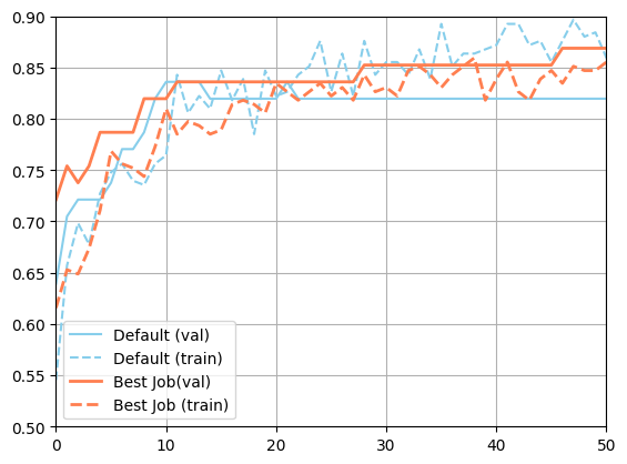
We can observe an improvement of more than 3% in accuracy. We can retrieve the corresponding hyperparameter configuration with the number of epochs used for this evaluation (32).

plt.figure(figsize=(40, 2))
cumulated_budget = 1
for i, job in results.iterrows():
    val_accuracy = json.loads(job["m:val_accuracy"])
    x = np.arange(len(val_accuracy)) + cumulated_budget
    cumulated_budget += len(val_accuracy)
    plt.plot(x, val_accuracy, label=f"Job {i}")
plt.ylabel("Validation Accuracy")
plt.xlabel("Cumulated Epochs")
plt.ylim(0.75, 0.9)
plt.grid()
plt.show()