5. Black-Box Multi-Objective Optimiaztion with DeepHyper (Basic)

In this tutorial, we will explore how to run black-box multi-objective optimization (MOO). In this setting, the goal is to resolve the following problem:

\[\text{max}_x (f_0(x), f_1(x), ..., f_n(x))\]

where \(x\) is the set of optimized variables and \(f_i\) are the different objectives. In DeepHyper, we use scalarization to transform such multi-objective problem into a single-objective problem:

\[\text{max}_x s_w((f_0(x), f_1(x), ..., f_n(x)))\]

where \(w\) is a set of weights which manages the trade-off between objectives and \(s_w : \mathbb{R}^n \rightarrow \mathbb{R}\). The weight vector \(w\) is randomized and re-sampled for each new batch of suggestion from the optimizer.

# Installing DeepHyper if not present
try:
    import deephyper
    print(deephyper.__version__)
except (ImportError, ModuleNotFoundError):
    !pip install deephyper

# Installing DeepHyper/Benchmark if not present
try:
    import deephyper_benchmark as dhb
except (ImportError, ModuleNotFoundError):
    !pip install -e "git+https://github.com/deephyper/benchmark.git@main#egg=deephyper-benchmark"

0.6.0

We will look at the DTLZ benchmark suite, a classic in multi-objective optimization (MOO) litterature. This benchmark exibit some characteristic cases of MOO. By default, this tutorial is loading the DTLZ-II benchmark which exibit a Pareto-Front with a concave shape.

import os

n_objectives = 2

# Configuration of the DTLZ Benchmark
os.environ["DEEPHYPER_BENCHMARK_DTLZ_PROB"] = str(2)
os.environ["DEEPHYPER_BENCHMARK_NDIMS"] = str(8)
os.environ["DEEPHYPER_BENCHMARK_NOBJS"] = str(n_objectives)
os.environ["DEEPHYPER_BENCHMARK_DTLZ_OFFSET"] = str(0.6)
os.environ["DEEPHYPER_BENCHMARK_FAILURES"] = str(0)

# Loading the DTLZ Benchmark
import deephyper_benchmark as dhb; dhb.load("DTLZ");
from deephyper_benchmark.lib.dtlz import hpo, metrics

/Users/romainegele/Documents/Argonne/deephyper/deephyper/problem/__init__.py:8: DeprecationWarning: The ``deephyper.problem`` module is deprecated, use ``deephyper.hpo`` instead.
  deprecated_api(__doc__)

We can display the variable search space of the benchmark we just loaded:

hpo.problem

Configuration space object:
  Hyperparameters:
    x0, Type: UniformFloat, Range: [0.0, 1.0], Default: 0.5
    x1, Type: UniformFloat, Range: [0.0, 1.0], Default: 0.5
    x2, Type: UniformFloat, Range: [0.0, 1.0], Default: 0.5
    x3, Type: UniformFloat, Range: [0.0, 1.0], Default: 0.5
    x4, Type: UniformFloat, Range: [0.0, 1.0], Default: 0.5
    x5, Type: UniformFloat, Range: [0.0, 1.0], Default: 0.5
    x6, Type: UniformFloat, Range: [0.0, 1.0], Default: 0.5
    x7, Type: UniformFloat, Range: [0.0, 1.0], Default: 0.5

To define a black-box for multi-objective optimization it is very similar to single-objective optimization at the difference that the objective can now be a list of values. A first possibility is:

def run(job):
    ...
    return objective_0, objective_1, ..., objective_n

which just returns the objectives to optimize as a tuple. If additionnal metadata are interesting to gather for each evaluation it is also possible to return them by following this format:

def run(job):
    ...
    return {
        "objective": [objective_0, objective_1, ..., objective_n],
        "metadata": {
            "flops": ...,
            "memory_footprint": ...,
            "duration": ...,
        }
    }

each of the metadata needs to be JSON serializable and will be returned in the final results with a column name formatted as m:metadata_key such as m:duration.

Now we can load Centralized Bayesian Optimization search:

from deephyper.hpo import CBO
from deephyper.evaluator import Evaluator
from deephyper.evaluator.callback import TqdmCallback

# Interface to submit/gather parallel evaluations of the black-box function.
# The method argument is used to specify the parallelization method, in our case we use threads.
# The method_kwargs argument is used to specify the number of workers and the callbacks.
# The TqdmCallback is used to display a progress bar during the search.
evaluator = Evaluator.create(
    hpo.run,
    method="thread",
    method_kwargs={"num_workers": 4, "callbacks": [TqdmCallback()]},
)

# Search algorithm
# The acq_func argument is used to specify the acquisition function.
# The multi_point_strategy argument is used to specify the multi-point strategy,
# in our case we use qUCB instead of the default cl_max (constant-liar) to reduce overheads.
# The update_prior argument is used to specify whether the sampling-prior should
# be updated during the search.
# The update_prior_quantile argument is used to specify the quantile of the lower-bound
# used to update the sampling-prior.
# The moo_scalarization_strategy argument is used to specify the scalarization strategy.
# Chebyshev is capable of generating a diverse set of solutions for non-convex problems.
# The moo_scalarization_weight argument is used to specify the weight of the scalarization.
# random is used to generate a random weight vector for each iteration.
search = CBO(
    hpo.problem,
    evaluator,
    acq_func="UCBd",
    multi_point_strategy="qUCB",
    acq_optimizer="ga",
    acq_optimizer_freq=1,
    moo_scalarization_strategy="AugChebyshev",
    moo_scalarization_weight="random",
    objective_scaler="identity",
    n_jobs=-1,
    verbose=1,
)

# Launch the search for a given number of evaluations
# other stopping criteria can be used (e.g. timeout, early-stopping/convergence)
results = search.search(max_evals=500)

WARNING:root:Results file already exists, it will be renamed to /Users/romainegele/Documents/Argonne/deephyper-tutorials/tutorials/colab/results_20240805-174730.csv

A Pandas table of results is returned by the search and also saved at ./results.csv. An other location can be specified by using CBO(..., log_dir=...).

results

	p:x0	p:x1	p:x2	p:x3	p:x4	p:x5	p:x6	p:x7	objective_0	objective_1	job_id	m:timestamp_submit	m:timestamp_start	m:timestamp_end	m:timestamp_gather	pareto_efficient
0	0.145748	0.357656	0.175772	0.679722	0.048408	0.144980	0.574257	0.034378	-2.022751	-0.471352	3	0.039462	1.722873e+09	1.722873e+09	0.040350	False
1	0.092662	0.413467	0.360699	0.817940	0.256936	0.796392	0.316346	0.161969	-1.551569	-0.227445	1	0.039446	1.722873e+09	1.722873e+09	0.043541	False
2	0.231148	0.925067	0.898563	0.897549	0.598821	0.771974	0.479363	0.495698	-1.251098	-0.475331	2	0.039454	1.722873e+09	1.722873e+09	0.043676	False
3	0.747343	0.125177	0.508432	0.861655	0.190644	0.790803	0.032897	0.191883	-0.770927	-1.839428	0	0.039435	1.722873e+09	1.722873e+09	0.043829	False
4	0.988159	0.330476	0.240062	0.381410	0.586152	0.535403	0.066100	0.220615	-0.031308	-1.683035	6	0.104634	1.722873e+09	1.722873e+09	0.105291	False
...	...	...	...	...	...	...	...	...	...	...	...	...	...	...	...	...
495	0.559597	0.801354	0.678211	0.841922	0.971817	0.507562	0.532400	0.838639	-0.837895	-1.011538	495	142.736880	1.722873e+09	1.722873e+09	142.737992	False
496	0.952890	0.458942	0.707773	0.783590	0.259506	0.886034	0.014616	0.269646	-0.126777	-1.710084	496	143.849656	1.722873e+09	1.722873e+09	143.850281	False
497	0.989093	0.595701	0.734708	0.996593	0.353719	0.652264	0.409195	0.560943	-0.021874	-1.276581	498	143.849681	1.722873e+09	1.722873e+09	143.850747	False
498	0.632611	0.019533	0.024721	0.444719	0.904616	0.914961	0.071286	0.660187	-1.182378	-1.816186	497	143.849669	1.722873e+09	1.722873e+09	143.850928	False
499	0.632611	0.019533	0.024721	0.444719	0.904616	0.914961	0.071286	0.660187	-1.182378	-1.816186	499	143.849688	1.722873e+09	1.722873e+09	143.851057	False

500 rows × 16 columns

In this table we retrieve:

• columns starting by p: which are the optimized variables.

• the objective_{i} are the objectives returned by the black-box function.

• the job_id is the identifier of the executed evaluations.

• columns starting by m: are metadata returned by the black-box function.

• pareto_efficient is a column only returned for MOO which specify if the evaluation is part of the set of optimal solutions.

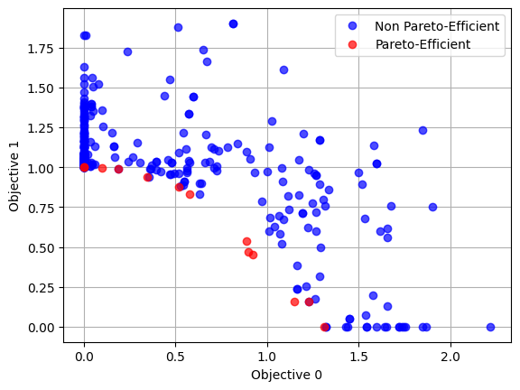
Let us use this table to visualized evaluated objectives:

import matplotlib.pyplot as plt

plt.figure()
plt.plot(
    -results[~results["pareto_efficient"]]["objective_0"],
    -results[~results["pareto_efficient"]]["objective_1"],
    "o",
    color="blue",
    alpha=0.7,
    label="Non Pareto-Efficient",
)
plt.plot(
    -results[results["pareto_efficient"]]["objective_0"],
    -results[results["pareto_efficient"]]["objective_1"],
    "o",
    color="red",
    alpha=0.7,
    label="Pareto-Efficient",
)
plt.grid()
plt.legend()
plt.xlabel("Objective 0")
plt.ylabel("Objective 1")
plt.show()