
Note
Go to the end to download the full example code.
Hyperparameter Optimization for Text Classification with Early Discarding#
Author(s): Romain Egele, Brett Eiffert.
In this example, we will edit the DeepHyper Hyperparameter Search for Text Classification example to use the
deephyper.stoppermodule. The Stopper class is used to check if training per job/evaluation can be ended early and save run time if the stopper algorithm determines that no more training is needed. Read more about the Stopper class here
Reference: This example is based on materials from the Pytorch Documentation: Text classification with the torchtext library
%%bash
pip install deephyper ray numpy==1.26.4 torch torchtext==0.17.2 torchdata==0.7.1 'portalocker>=2.0.0'
Imports#
All imports used in the tutorial are declared at the top of the file.
Code (Imports)
from deephyper.evaluator import RunningJob

import ray
import json
from functools import partial

import torch

from torchtext.data.utils import get_tokenizer
from torchtext.data.functional import to_map_style_dataset
from torchtext.vocab import build_vocab_from_iterator
from torchtext.datasets import AG_NEWS

from torch.utils.data import DataLoader
from torch.utils.data.dataset import random_split

from torch import nn
Note
The following can be used to detect if CUDA devices are available on the current host. Therefore, this notebook will automatically adapt the parallel execution based on the resources available locally. However, it will not be the case if many compute nodes are requested.
If GPU is available, this code will enabled the tutorial to use the GPU for pytorch operations.
Code (Code to check if using CPU or GPU)
The dataset#
The torchtext library provides a few raw dataset iterators, which yield the raw text strings. For example, the AG_NEWS dataset iterators yield the raw data as a tuple of label and text. It has four labels (1 : World 2 : Sports 3 : Business 4 : Sci/Tec).
Code (Loading the data)
def load_data(train_ratio, fast=False):
    train_iter, test_iter = AG_NEWS()
    train_dataset = to_map_style_dataset(train_iter)
    test_dataset = to_map_style_dataset(test_iter)
    num_train = int(len(train_dataset) * train_ratio)
    split_train, split_valid = \
        random_split(train_dataset, [num_train, len(train_dataset) - num_train])

    ## downsample
    if fast:
        split_train, _ = random_split(split_train, [int(len(split_train)*.05), int(len(split_train)*.95)])
        split_valid, _ = random_split(split_valid, [int(len(split_valid)*.05), int(len(split_valid)*.95)])
        test_dataset, _ = random_split(test_dataset, [int(len(test_dataset)*.05), int(len(test_dataset)*.95)])

    return split_train, split_valid, test_dataset
Preprocessing pipelines and Batch generation#
Here is an example for typical NLP data processing with tokenizer and vocabulary. The first step is to build a vocabulary with the raw training dataset. Here we use built in
factory function build_vocab_from_iterator which accepts iterator that yield list or iterator of tokens. Users can also pass any special symbols to be added to the
vocabulary.
The vocabulary block converts a list of tokens into integers.
vocab(['here', 'is', 'an', 'example'])
>>> [475, 21, 30, 5286]
The text pipeline converts a text string into a list of integers based on the lookup table defined in the vocabulary. The label pipeline converts the label into integers. For example,
text_pipeline('here is the an example')
>>> [475, 21, 2, 30, 5286]
label_pipeline('10')
>>> 9
Code (Code to tokenize and build vocabulary for text processing)
train_iter = AG_NEWS(split='train')
num_class = 4

tokenizer = get_tokenizer('basic_english')

def yield_tokens(data_iter):
    for _, text in data_iter:
        yield tokenizer(text)

vocab = build_vocab_from_iterator(yield_tokens(train_iter), specials=["<unk>"])
vocab.set_default_index(vocab["<unk>"])
vocab_size = len(vocab)

text_pipeline = lambda x: vocab(tokenizer(x))
label_pipeline = lambda x: int(x) - 1


def collate_batch(batch, device):
    label_list, text_list, offsets = [], [], [0]
    for (_label, _text) in batch:
        label_list.append(label_pipeline(_label))
        processed_text = torch.tensor(text_pipeline(_text), dtype=torch.int64)
        text_list.append(processed_text)
        offsets.append(processed_text.size(0))
    label_list = torch.tensor(label_list, dtype=torch.int64)
    offsets = torch.tensor(offsets[:-1]).cumsum(dim=0)
    text_list = torch.cat(text_list)
    return label_list.to(device), text_list.to(device), offsets.to(device)
Note
The collate_fn function works on a batch of samples generated from DataLoader. The input to collate_fn is a batch of data with the batch size in DataLoader, and collate_fn processes them according to the data processing pipelines declared previously.
Define the model#
The model is composed of the nn.EmbeddingBag layer plus a linear layer for the classification purpose.
Code (Defining the Text Classification model)
class TextClassificationModel(nn.Module):

    def __init__(self, vocab_size, embed_dim, num_class):
        super().__init__()
        self.embedding = nn.EmbeddingBag(vocab_size, embed_dim, sparse=False)
        self.fc = nn.Linear(embed_dim, num_class)
        self.init_weights()

    def init_weights(self):
        initrange = 0.5
        self.embedding.weight.data.uniform_(-initrange, initrange)
        self.fc.weight.data.uniform_(-initrange, initrange)
        self.fc.bias.data.zero_()

    def forward(self, text, offsets):
        embedded = self.embedding(text, offsets)
        return self.fc(embedded)
Define functions to train the model and evaluate results.#
Code (Define the training and evaluation of the Text Classification model)
def train(model, criterion, optimizer, dataloader):
    model.train()

    for _, (label, text, offsets) in enumerate(dataloader):
        optimizer.zero_grad()
        predicted_label = model(text, offsets)
        loss = criterion(predicted_label, label)
        loss.backward()
        torch.nn.utils.clip_grad_norm_(model.parameters(), 0.1)
        optimizer.step()

def evaluate(model, dataloader):
    model.eval()
    total_acc, total_count = 0, 0

    with torch.no_grad():
        for _, (label, text, offsets) in enumerate(dataloader):
            predicted_label = model(text, offsets)
            total_acc += (predicted_label.argmax(1) == label).sum().item()
            total_count += label.size(0)
    return total_acc/total_count
Define the run-function#
The run-function defines how the objective that we want to maximize is computed. It takes a config dictionary as input and often returns a scalar value that we want to maximize. The config contains a sample value of hyperparameters that we want to tune. In this example we will search for:
num_epochs(default value:10)batch_size(default value:64)learning_rate(default value:5)
A hyperparameter value can be accessed easily in the dictionary through the corresponding key, for example config["units"].
When a Stopper is defined and set as a parameter in a search (below CBO()`),
the run function must invoke methods job.record() and job.stopped().
job.record() tells the Stopper which values to watch so it knows to stop
and then job.stopped() is a state the stopper uses to exit the specific job in the search earlier than expected.
def get_run(train_ratio=0.95):
  def run(job: RunningJob):
    device = torch.device("cuda" if torch.cuda.is_available() else "cpu")

    embed_dim = 64
    num_epochs = 100

    collate_fn = partial(collate_batch, device=device)
    split_train, split_valid, _ = load_data(train_ratio, fast=True) # set fast=false for longer running, more accurate example
    train_dataloader = DataLoader(split_train, batch_size=int(job["batch_size"]),
                                shuffle=True, collate_fn=collate_fn)
    valid_dataloader = DataLoader(split_valid, batch_size=int(job["batch_size"]),
                                shuffle=True, collate_fn=collate_fn)

    model = TextClassificationModel(vocab_size, int(embed_dim), num_class).to(device)

    criterion = torch.nn.CrossEntropyLoss()
    optimizer = torch.optim.SGD(model.parameters(), lr=job["learning_rate"])

    accu_list = []
    for i in range(1, num_epochs + 1):
        train(model, criterion, optimizer, train_dataloader)
        accu_list.append(evaluate(model, valid_dataloader))
        job.record(budget = i + 1, objective=evaluate(model, valid_dataloader))
        if job.stopped():
            break

    accu_test = evaluate(model, valid_dataloader)
    return {"objective": accu_test, "metadata": {"index_stopped": i, "accu_list": accu_list}}
  return run
We create two versions of run, one quicker to evaluate for the search, with a small training dataset, and another one, for performance evaluation, which uses a normal training/validation ratio.
quick_run = get_run(train_ratio=0.3)
perf_run = get_run(train_ratio=0.95)
Note
The objective maximised by DeepHyper is the scalar value returned by the run-function.
In this tutorial it corresponds to the validation accuracy of the model after training.
Define the Hyperparameter optimization problem#
Hyperparameter ranges are defined using the following syntax:
Discrete integer ranges are generated from a tuple
(lower: int, upper: int)Continuous prarameters are generated from a tuple
(lower: float, upper: float)Categorical or nonordinal hyperparameter ranges can be given as a list of possible values
[val1, val2, ...]
We provide the default configuration of hyperparameters as a starting point of the problem.
from deephyper.hpo import HpProblem

problem = HpProblem()

# Discrete and Real hyperparameters (sampled with log-uniform)
problem.add_hyperparameter((8, 512, "log-uniform"), "batch_size", default_value=64)
problem.add_hyperparameter((0.1, 10, "log-uniform"), "learning_rate", default_value=5)

problem
Configuration space object:
  Hyperparameters:
    batch_size, Type: UniformInteger, Range: [8, 512], Default: 64, on log-scale
    learning_rate, Type: UniformFloat, Range: [0.1, 10.0], Default: 5.0, on log-scale
Evaluate a default configuration#
We evaluate the performance of the default set of hyperparameters provided in the Pytorch tutorial.
Code (Imports)
#We launch the Ray run-time and execute the `run` function
#with the default configuration

if is_gpu_available:
    if not(ray.is_initialized()):
        ray.init(num_cpus=n_gpus, num_gpus=n_gpus, log_to_driver=False)

    run_default = ray.remote(num_cpus=1, num_gpus=1)(perf_run)
    objective_default = ray.get(run_default.remote(RunningJob(parameters=problem.default_configuration)))
else:
    if not(ray.is_initialized()):
        ray.init(num_cpus=1, log_to_driver=False)
    run_default = perf_run
    objective_default = run_default(RunningJob(parameters=problem.default_configuration))
    print(problem.default_configuration)

print(f"Accuracy Default Configuration:  {objective_default["objective"]:.3f}")
2025-10-21 16:04:22,173 INFO worker.py:1843 -- Started a local Ray instance. View the dashboard at http://127.0.0.1:8265
{'batch_size': 64, 'learning_rate': 5.0}
Accuracy Default Configuration:  0.887
Define the evaluator object#
The Evaluator object allows to change the parallelization backend used by DeepHyper.
It is a standalone object which schedules the execution of remote tasks. All evaluators needs a run_function to be instantiated.
Then a keyword method defines the backend (e.g., "ray") and the method_kwargs corresponds to keyword arguments of this chosen method.
evaluator = Evaluator.create(run_function, method, method_kwargs)
Once created the evaluator.num_workers gives access to the number of available parallel workers.
Finally, to submit and collect tasks to the evaluator one just needs to use the following interface:
Warning
Each Evaluator saves its own state, therefore it is crucial to create a new evaluator when launching a fresh search.
Code (Imports)
from deephyper.evaluator import Evaluator
from deephyper.evaluator.callback import TqdmCallback


def get_evaluator(run_function):
    # Default arguments for Ray: 1 worker and 1 worker per evaluation
    method_kwargs = {
        "num_cpus": 1,
        "num_cpus_per_task": 1,
        "callbacks": [TqdmCallback()]
    }

    # If GPU devices are detected then it will create 'n_gpus' workers
    # and use 1 worker for each evaluation
    if is_gpu_available:
        method_kwargs["num_cpus"] = n_gpus
        method_kwargs["num_gpus"] = n_gpus
        method_kwargs["num_cpus_per_task"] = 1
        method_kwargs["num_gpus_per_task"] = 1

    evaluator = Evaluator.create(
        run_function,
        method="ray",
        method_kwargs=method_kwargs
    )
    print(f"Created new evaluator with {evaluator.num_workers} worker{'s' if evaluator.num_workers > 1 else ''} and config: {method_kwargs}", )

    return evaluator

evaluator = get_evaluator(quick_run)
Created new evaluator with 1 worker and config: {'num_cpus': 1, 'num_cpus_per_task': 1, 'callbacks': [<deephyper.evaluator.callback.TqdmCallback object at 0x3a4eedd60>]}
Define and run the Centralized Bayesian Optimization search (CBO)#
We create the CBO using the problem and evaluator defined above.
A Stopper is also defined and passed as an argument to the CBO. This Stopper controls the job.observe() and job.stopped() functions.
from deephyper.hpo import CBO
from deephyper.stopper import SuccessiveHalvingStopper
Instantiate the search with the problem and a specific evaluator
Results file already exists, it will be renamed to /Users/rp5/Documents/DeepHyper/deephyper/examples/examples_hpo/stopper-log-files/results_20251021-160501.csv
Note
- All DeepHyper’s search algorithm have two stopping criteria:
max_evals (int): Defines the maximum number of evaluations that we want to perform. Default to-1for an infinite number.timeout (int): Defines a time budget (in seconds) before stopping the search. Default toNonefor an infinite time budget.
results = search.search(evaluator, max_evals=30)
  0%|          | 0/30 [00:00<?, ?it/s]
  3%|▎         | 1/30 [00:00<00:00, 5210.32it/s, failures=0, objective=0.729]
  7%|▋         | 2/30 [01:00<14:06, 30.25s/it, failures=0, objective=0.729]
  7%|▋         | 2/30 [01:00<14:06, 30.25s/it, failures=0, objective=0.787]
 10%|█         | 3/30 [01:36<14:42, 32.70s/it, failures=0, objective=0.787]
 10%|█         | 3/30 [01:36<14:42, 32.70s/it, failures=0, objective=0.808]
 13%|█▎        | 4/30 [01:37<09:00, 20.79s/it, failures=0, objective=0.808]
 13%|█▎        | 4/30 [01:37<09:00, 20.79s/it, failures=0, objective=0.808]
 17%|█▋        | 5/30 [02:32<13:40, 32.83s/it, failures=0, objective=0.808]
 17%|█▋        | 5/30 [02:32<13:40, 32.83s/it, failures=0, objective=0.81]
 20%|██        | 6/30 [02:34<08:56, 22.34s/it, failures=0, objective=0.81]
 20%|██        | 6/30 [02:34<08:56, 22.34s/it, failures=0, objective=0.81]
 23%|██▎       | 7/30 [02:36<06:04, 15.85s/it, failures=0, objective=0.81]
 23%|██▎       | 7/30 [02:36<06:04, 15.85s/it, failures=0, objective=0.81]
 27%|██▋       | 8/30 [02:37<04:08, 11.31s/it, failures=0, objective=0.81]
 27%|██▋       | 8/30 [02:37<04:08, 11.31s/it, failures=0, objective=0.81]
 30%|███       | 9/30 [02:40<02:59,  8.54s/it, failures=0, objective=0.81]
 30%|███       | 9/30 [02:40<02:59,  8.54s/it, failures=0, objective=0.81]
 33%|███▎      | 10/30 [02:41<02:06,  6.34s/it, failures=0, objective=0.81]
 33%|███▎      | 10/30 [02:41<02:06,  6.34s/it, failures=0, objective=0.81]
 37%|███▋      | 11/30 [02:42<01:30,  4.74s/it, failures=0, objective=0.81]
 37%|███▋      | 11/30 [02:42<01:30,  4.74s/it, failures=0, objective=0.81]
 40%|████      | 12/30 [02:43<01:05,  3.66s/it, failures=0, objective=0.81]
 40%|████      | 12/30 [02:43<01:05,  3.66s/it, failures=0, objective=0.81]
 43%|████▎     | 13/30 [02:45<00:50,  2.96s/it, failures=0, objective=0.81]
 43%|████▎     | 13/30 [02:45<00:50,  2.96s/it, failures=0, objective=0.81]
 47%|████▋     | 14/30 [02:46<00:40,  2.54s/it, failures=0, objective=0.81]
 47%|████▋     | 14/30 [02:46<00:40,  2.54s/it, failures=0, objective=0.81]
 50%|█████     | 15/30 [02:47<00:31,  2.12s/it, failures=0, objective=0.81]
 50%|█████     | 15/30 [02:47<00:31,  2.12s/it, failures=0, objective=0.81]
 53%|█████▎    | 16/30 [02:48<00:25,  1.84s/it, failures=0, objective=0.81]
 53%|█████▎    | 16/30 [02:48<00:25,  1.84s/it, failures=0, objective=0.81]
 57%|█████▋    | 17/30 [02:50<00:21,  1.64s/it, failures=0, objective=0.81]
 57%|█████▋    | 17/30 [02:50<00:21,  1.64s/it, failures=0, objective=0.81]
 60%|██████    | 18/30 [02:53<00:27,  2.25s/it, failures=0, objective=0.81]
 60%|██████    | 18/30 [02:53<00:27,  2.25s/it, failures=0, objective=0.81]
 63%|██████▎   | 19/30 [02:54<00:21,  1.91s/it, failures=0, objective=0.81]
 63%|██████▎   | 19/30 [02:54<00:21,  1.91s/it, failures=0, objective=0.81]
 67%|██████▋   | 20/30 [02:56<00:16,  1.68s/it, failures=0, objective=0.81]
 67%|██████▋   | 20/30 [02:56<00:16,  1.68s/it, failures=0, objective=0.81]
 70%|███████   | 21/30 [02:58<00:17,  1.96s/it, failures=0, objective=0.81]
 70%|███████   | 21/30 [02:58<00:17,  1.96s/it, failures=0, objective=0.81]
 73%|███████▎  | 22/30 [03:43<01:59, 14.89s/it, failures=0, objective=0.81]
 73%|███████▎  | 22/30 [03:43<01:59, 14.89s/it, failures=0, objective=0.81]
 77%|███████▋  | 23/30 [03:45<01:17, 11.05s/it, failures=0, objective=0.81]
 77%|███████▋  | 23/30 [03:45<01:17, 11.05s/it, failures=0, objective=0.81]
 80%|████████  | 24/30 [03:47<00:48,  8.16s/it, failures=0, objective=0.81]
 80%|████████  | 24/30 [03:47<00:48,  8.16s/it, failures=0, objective=0.81]
 83%|████████▎ | 25/30 [03:48<00:30,  6.15s/it, failures=0, objective=0.81]
 83%|████████▎ | 25/30 [03:48<00:30,  6.15s/it, failures=0, objective=0.81]
 87%|████████▋ | 26/30 [03:50<00:19,  4.89s/it, failures=0, objective=0.81]
 87%|████████▋ | 26/30 [03:50<00:19,  4.89s/it, failures=0, objective=0.81]
 90%|█████████ | 27/30 [03:51<00:11,  3.76s/it, failures=0, objective=0.81]
 90%|█████████ | 27/30 [03:51<00:11,  3.76s/it, failures=0, objective=0.81]
 93%|█████████▎| 28/30 [03:53<00:06,  3.09s/it, failures=0, objective=0.81]
 93%|█████████▎| 28/30 [03:53<00:06,  3.09s/it, failures=0, objective=0.81]
 97%|█████████▋| 29/30 [03:54<00:02,  2.53s/it, failures=0, objective=0.81]
 97%|█████████▋| 29/30 [03:54<00:02,  2.53s/it, failures=0, objective=0.81]
100%|██████████| 30/30 [03:55<00:00,  2.19s/it, failures=0, objective=0.81]
100%|██████████| 30/30 [03:55<00:00,  2.19s/it, failures=0, objective=0.81]
100%|██████████| 30/30 [03:55<00:00,  7.86s/it, failures=0, objective=0.81]
The returned results is a Pandas Dataframe where columns are hyperparameters and information stored by the evaluator:
job_idis a unique identifier corresponding to the order of creation of tasksobjectiveis the value returned by the run-functiontimestamp_submitis the time (in seconds) when the hyperparameter configuration was submitted by theEvaluatorrelative to the creation of the evaluator.timestamp_gatheris the time (in seconds) when the hyperparameter configuration was collected by theEvaluatorrelative to the creation of the evaluator.
Show results. As shown by the index_stopped column, even there were 100 epochs per job, not all jobs used all 100 epochs.
The power of a Stopper is shown as it can reduce runtime significantly as the Stopper and jobs become “smart” and decide to end early
because the Stopper algorithm determined it was unnecessary to move forward in the search for that job.
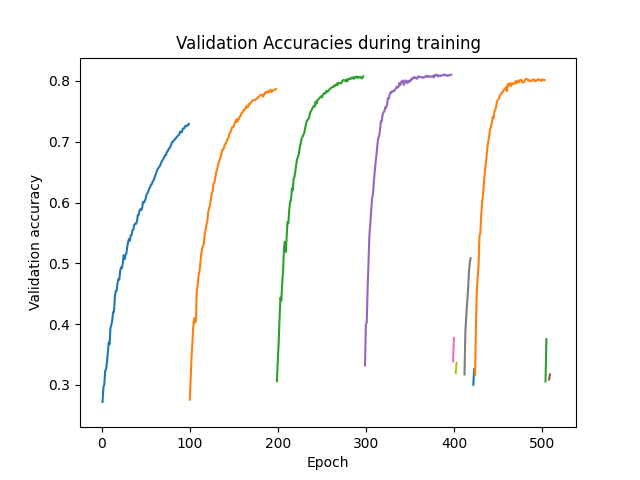
Visualizing the Stopper#
This graph shows the same information as described above but in a visual form. Each of the 30 jobs and the rate at which they learned against the validation dataset is shown here. As shown above, not all job lines will show 100 epochs because the Stopper determined the jobs did not need to run the full time to converge on a solution.
import numpy as np
import matplotlib.pyplot as plt

i = 0
for row in results.iterrows():
    y = row[1]["m:accu_list"]
    x = np.arange(i+1, i+1+len(y))
    plt.plot(x, y, label=row[1]["job_id"])
    i += len(y)

plt.xlabel('Epoch')
plt.ylabel('Validation accuracy')
plt.title("Validation Accuracies during training")

plt.show()
Evaluate the best configuration#
Now that the search is over, let us print the best configuration found during this run and evaluate it on the full training dataset.
Show the job with best configuration and compare this with the graph above. The result of the comparison should be intuitive -
the job with the best objective in the graph should match i_max.
4
best_config = results.iloc[i_max][:-3].to_dict()
best_config = {k[2:]: v for k, v in best_config.items() if k.startswith("p:")}

print(f"The default configuration has an accuracy of {objective_default["objective"]:.3f}. \n"
      f"The best configuration found by DeepHyper has an accuracy {results['objective'].iloc[i_max]:.3f}, \n"
      f"finished after {results['m:timestamp_gather'].iloc[i_max]:.2f} seconds of search.\n")

print(json.dumps(best_config, indent=4))
The default configuration has an accuracy of 0.887.
The best configuration found by DeepHyper has an accuracy 0.810,
finished after 183.35 seconds of search.

{
    "batch_size": 14,
    "learning_rate": 0.8747246682101409
}
objective_best = perf_run(RunningJob(parameters=best_config))
print(f"Accuracy Best Configuration:  {objective_best["objective"]:.3f}")
Accuracy Best Configuration: 0.867
Total running time of the script: (7 minutes 49.357 seconds)