Profile the Worker Utilization

Author(s): Romain Egele.

In this example, you will learn how to profile the activity of workers during a search.

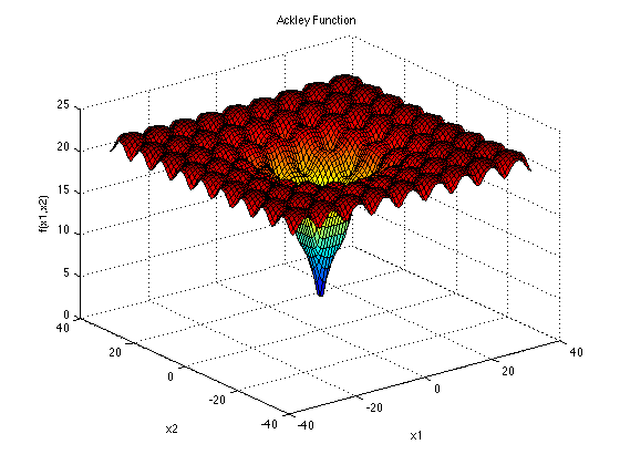
We start by defining an artificial black-box run-function by using the Ackley function:

Code (Import statements)

import time

import matplotlib.pyplot as plt
import numpy as np

from deephyper.analysis import figure_size
from deephyper.analysis.hpo import (
    plot_search_trajectory_single_objective_hpo,
    plot_worker_utilization,
)
from deephyper.evaluator import Evaluator, profile
from deephyper.evaluator.callback import TqdmCallback
from deephyper.hpo import CBO, HpProblem

We define the Ackley function:

Code (Ackley function)

def ackley(x, a=20, b=0.2, c=2 * np.pi):
    d = len(x)
    s1 = np.sum(x**2)
    s2 = np.sum(np.cos(c * x))
    term1 = -a * np.exp(-b * np.sqrt(s1 / d))
    term2 = -np.exp(s2 / d)
    y = term1 + term2 + a + np.exp(1)
    return y

We will use the time.sleep function to simulate a budget of 2 secondes of execution in average which helps illustrate the advantage of parallel evaluations. The @profile decorator is useful to collect starting/ending time of the run-function execution which help us know exactly when we are inside the black-box. This decorator is necessary when profiling the worker utilization. When using this decorator, the run-function will return a dictionnary with 2 new keys "timestamp_start" and "timestamp_end".

@profile
def run_ackley(config, sleep_loc=2, sleep_scale=0.5):
    # to simulate the computation of an expensive black-box
    if sleep_loc > 0:
        t_sleep = np.random.normal(loc=sleep_loc, scale=sleep_scale)
        t_sleep = max(t_sleep, 0)
        time.sleep(t_sleep)

    x = np.array([config[k] for k in config if "x" in k])
    x = np.asarray_chkfinite(x)  # ValueError if any NaN or Inf
    return -ackley(x)  # maximisation is performed

Then we define the variable(s) we want to optimize. For this problem we optimize Ackley in a 2-dimensional search space, the true minimul is located at (0, 0).

def create_problem(nb_dim=2):
    nb_dim = 2
    problem = HpProblem()
    for i in range(nb_dim):
        problem.add_hyperparameter((-32.768, 32.768), f"x{i}")
    return problem

problem = create_problem()
problem

Configuration space object:
  Hyperparameters:
    x0, Type: UniformFloat, Range: [-32.768, 32.768], Default: 0.0
    x1, Type: UniformFloat, Range: [-32.768, 32.768], Default: 0.0

Then we define a parallel search.

As the run-function is defined in the same module we use the “loky” backend

that serialize by value.

def execute_search(timeout, num_workers):

    evaluator = Evaluator.create(
        run_ackley,
        method="loky",
        method_kwargs={
            "num_workers": num_workers,
            "callbacks": [TqdmCallback()],
        },
    )

    search = CBO(
        problem,
        evaluator,
        multi_point_strategy="qUCBd",
        random_state=42,
    )

    results = search.search(timeout=timeout)

    return results

if __name__ == "__main__":
    timeout = 20
    num_workers = 4
    results = execute_search(timeout, num_workers)

0it [00:00, ?it/s]
1it [00:00, 4928.68it/s, failures=0, objective=-21.5]
2it [00:00, 61.69it/s, failures=0, objective=-19.8]
3it [00:00, 91.44it/s, failures=0, objective=-19.8]
4it [00:00,  5.36it/s, failures=0, objective=-19.8]
4it [00:00,  5.36it/s, failures=0, objective=-19.8]
5it [00:01,  4.24it/s, failures=0, objective=-19.8]
5it [00:01,  4.24it/s, failures=0, objective=-19.8]
6it [00:02,  1.66it/s, failures=0, objective=-19.8]
6it [00:02,  1.66it/s, failures=0, objective=-19.8]
7it [00:02,  1.96it/s, failures=0, objective=-19.8]
7it [00:02,  1.96it/s, failures=0, objective=-15.4]
8it [00:02,  1.96it/s, failures=0, objective=-15.4]
9it [00:03,  2.85it/s, failures=0, objective=-15.4]
9it [00:03,  2.85it/s, failures=0, objective=-15.4]
10it [00:04,  1.56it/s, failures=0, objective=-15.4]
10it [00:04,  1.56it/s, failures=0, objective=-12.6]
11it [00:05,  1.84it/s, failures=0, objective=-12.6]
11it [00:05,  1.84it/s, failures=0, objective=-12.6]
12it [00:05,  2.03it/s, failures=0, objective=-12.6]
12it [00:05,  2.03it/s, failures=0, objective=-12.6]
13it [00:05,  2.34it/s, failures=0, objective=-12.6]
13it [00:05,  2.34it/s, failures=0, objective=-12.6]
14it [00:07,  1.31it/s, failures=0, objective=-12.6]
14it [00:07,  1.31it/s, failures=0, objective=-12.6]
15it [00:07,  1.62it/s, failures=0, objective=-12.6]
15it [00:07,  1.62it/s, failures=0, objective=-4.19]
16it [00:07,  1.86it/s, failures=0, objective=-4.19]
16it [00:07,  1.86it/s, failures=0, objective=-4.19]
17it [00:08,  2.21it/s, failures=0, objective=-4.19]
17it [00:08,  2.21it/s, failures=0, objective=-4.19]
18it [00:09,  1.58it/s, failures=0, objective=-4.19]
18it [00:09,  1.58it/s, failures=0, objective=-4.19]
19it [00:09,  1.68it/s, failures=0, objective=-4.19]
19it [00:09,  1.68it/s, failures=0, objective=-2.17]
20it [00:10,  1.85it/s, failures=0, objective=-2.17]
20it [00:10,  1.85it/s, failures=0, objective=-2.17]
21it [00:10,  2.18it/s, failures=0, objective=-2.17]
21it [00:10,  2.18it/s, failures=0, objective=-2.17]
22it [00:11,  1.96it/s, failures=0, objective=-2.17]
22it [00:11,  1.96it/s, failures=0, objective=-0.729]
23it [00:11,  2.29it/s, failures=0, objective=-0.729]
23it [00:11,  2.29it/s, failures=0, objective=-0.729]
24it [00:12,  1.75it/s, failures=0, objective=-0.729]
24it [00:12,  1.75it/s, failures=0, objective=-0.729]
25it [00:12,  1.69it/s, failures=0, objective=-0.729]
25it [00:12,  1.69it/s, failures=0, objective=-0.729]
26it [00:13,  1.75it/s, failures=0, objective=-0.729]
26it [00:13,  1.75it/s, failures=0, objective=-0.729]
27it [00:13,  2.08it/s, failures=0, objective=-0.729]
27it [00:13,  2.08it/s, failures=0, objective=-0.729]
28it [00:14,  1.62it/s, failures=0, objective=-0.729]
28it [00:14,  1.62it/s, failures=0, objective=-0.729]
29it [00:15,  1.48it/s, failures=0, objective=-0.729]
29it [00:15,  1.48it/s, failures=0, objective=-0.729]
30it [00:15,  1.80it/s, failures=0, objective=-0.729]
30it [00:15,  1.80it/s, failures=0, objective=-0.729]
31it [00:15,  2.16it/s, failures=0, objective=-0.729]
31it [00:15,  2.16it/s, failures=0, objective=-0.729]
32it [00:17,  1.30it/s, failures=0, objective=-0.729]
32it [00:17,  1.30it/s, failures=0, objective=-0.729]
33it [00:18,  1.07it/s, failures=0, objective=-0.729]
33it [00:18,  1.07it/s, failures=0, objective=-0.729]
34it [00:18,  1.07it/s, failures=0, objective=-0.729]
35it [00:18,  1.07it/s, failures=0, objective=-0.729]

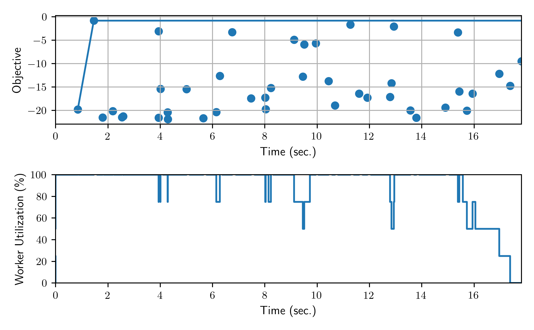
Finally, we plot the results from the collected DataFrame.

Code (Plot search trajectory an workers utilization)

if __name__ == "__main__":
    t0 = results["m:timestamp_start"].iloc[0]
    results["m:timestamp_start"] = results["m:timestamp_start"] - t0
    results["m:timestamp_end"] = results["m:timestamp_end"] - t0
    tmax = results["m:timestamp_end"].max()

    fig, axes = plt.subplots(
        nrows=2,
        ncols=1,
        sharex=True,
        figsize=figure_size(width=600),
        tight_layout=True,
    )

    _ = plot_search_trajectory_single_objective_hpo(
        results, mode="min", x_units="seconds", ax=axes[0],
    )

    _ = plot_worker_utilization(
        results, num_workers=num_workers, profile_type="start/end", ax=axes[1],
    )